One-sentence summary: Sparse Attention computes fewer connections, Linear Attention changes the similarity rule, and Infini-attention compresses old cross-segment K/V into bounded state—the three mechanisms solve different problems, and none preserves an unlimited history for free.
24.1 Full Attention has three separate bills
24.1.1 Connections
Full Self-Attention over length compares every Query with every Key. Bidirectional attention has connections. Causal attention permits the lower triangle:
“Only the lower triangle is logically valid” does not mean an ordinary dense matrix multiplication automatically skips the other half. Whether masked regions avoid real work depends on the kernel.
| Bidirectional | Valid causal | |
|---|---|---|
| 1,024 | 1,048,576 | 524,800 |
| 4,096 | 16,777,216 | 8,390,656 |
| 32,768 | 1,073,741,824 | 536,887,296 |
| 1,000,000 | 1,000,000,000,000 | 500,000,500,000 |
Make the sequence ten times longer and the number of connections becomes roughly one hundred times larger. That is the first bill: quadratic arithmetic.
24.1.2 Intermediate storage
If one Head's full score matrix were materialized in FP16 or BF16, it would occupy:
| Dense score matrix for one Head | |
|---|---|
| 4,096 | 32 MiB |
| 8,192 | 128 MiB |
| 32,768 | 2 GiB |
| 131,072 | 32 GiB |
Those figures describe one Head and one matrix, not an entire layer. Materializing every Head multiplies them by the Head count; training also needs state for backward.
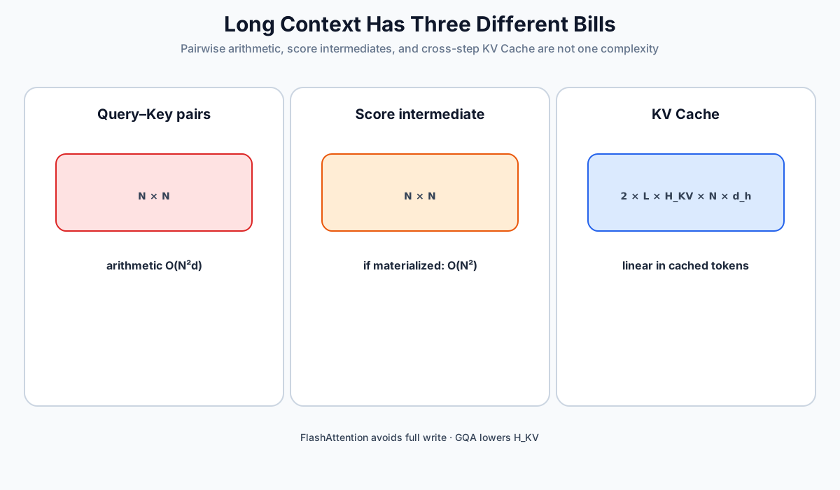
Chapter 21 showed why this table is no longer a requirement. FlashAttention computes exact Softmax Attention without writing the full score matrix to HBM. It reduces I/O and working storage toward linear growth in sequence length, but it still processes the quadratic set of Query–Key pairs.
24.1.3 KV Cache is a different axis
Chapter 23's KV Cache grows linearly with cached tokens; Full Attention's training or Prefill pairs grow quadratically. Keep the axes separate:
- FlashAttention avoids materializing the full score matrix while preserving Full Attention math;
- GQA/MQA reduce KV Heads and cache bytes;
- Sparse Attention removes allowed Query–Key connections;
- Linear Attention replaces the Softmax similarity computation;
- Infini-attention compresses history across segments while retaining exact local Attention inside the current segment.
Once these are separated, the complexity claims become much easier to audit.
24.2 Sparse Attention: draw the graph before writing O(N)
Imagine reading an annotated logbook from a remote Orkney lighthouse. The current entry is most likely to depend on nearby weather observations. The first entry of a storm can serve as a global anchor. A few links across months can shorten the path between distant events. Sparse Attention makes this “who may see whom” graph explicit.
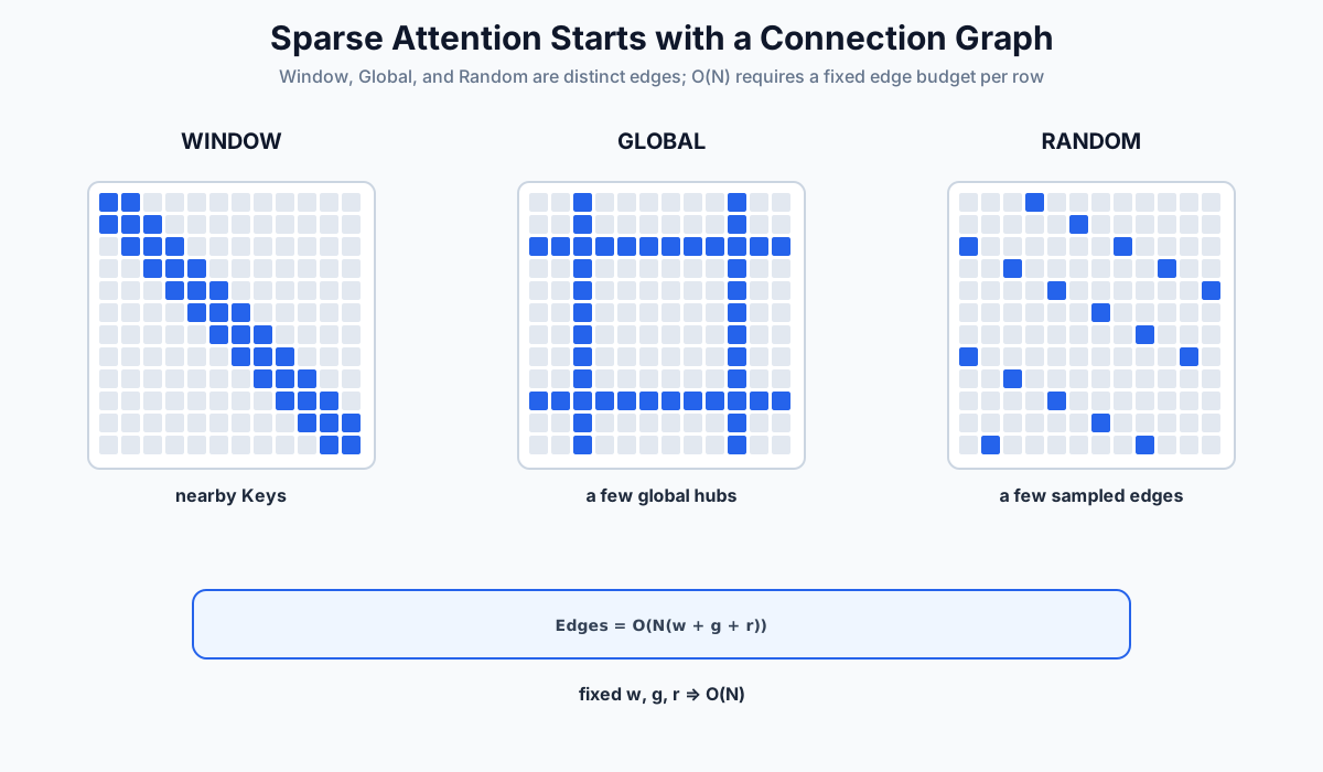
Three common edge types are:
- Window / Local: every Query sees roughly nearby Keys.
- Global: a small set of positions connects to the entire sequence in both directions, as with task-selected Longformer tokens.
- Random: each position adds randomly chosen links; BigBird combines these with Window and Global links.
If each row has a fixed number of these edges, the main edge count is:
This is abbreviated to only when remain fixed as grows. A window that grows with the sequence changes the complexity.
24.2.1 What Longformer and BigBird actually establish
Longformer combines a sliding window with task-selected global Attention. Its original work centered on long-document encoding, masked language modeling, and the LED encoder–decoder. BigBird adds random connections and likewise focused largely on BERT-style long-sequence encoding tasks.
The BigBird paper proves, under its graph construction and assumptions about global tokens, depth, and precision, that a sparse Transformer can retain universal-approximation and Turing-completeness properties. It does not prove that:
- an arbitrary random pattern connects any two tokens in a fixed number of layers;
- a finite, trained BigBird always matches Full Attention;
- accuracy loss is slight on every task.
Theoretical expressivity, graph path length, and trained-model quality are three different claims.
24.2.2 A mask is not a speedup
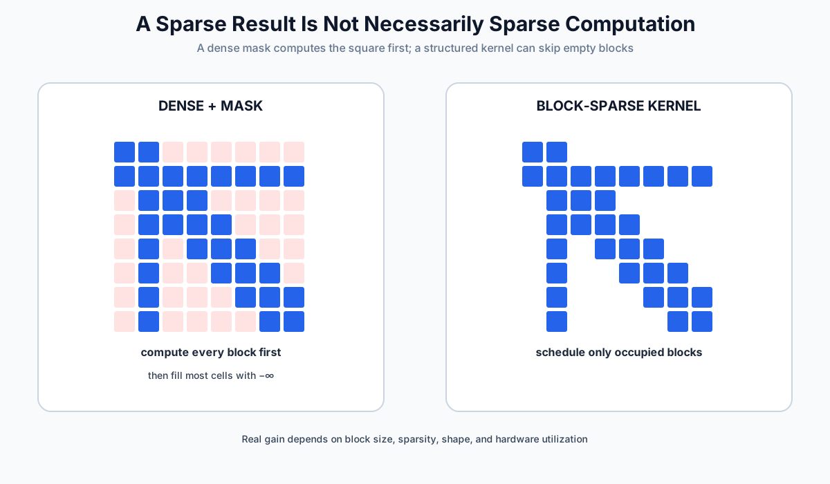
Filling a normal score matrix with -inf in disallowed cells gives the right Sparse Attention result, but the dense matrix has already been computed. Real savings require a structured block-sparse or FlexAttention-style kernel that skips empty blocks. Block size, sparsity, shape, and hardware utilization determine real speed; with too little useful sparsity, scheduling overhead can erase the theoretical gain.
24.3 Sliding Window: simple idea, easy off-by-one
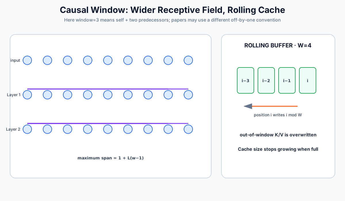
Consider a decoder's causal window. Here window=3 means that a position may see itself and its two immediate predecessors:
q0 -> k0
q1 -> k0 k1
q2 -> k0 k1 k2
q3 ->    k1 k2 k3
...
At length 8 there are not valid connections, but . Three links are missing at the left boundary.
import math
import torch


def causal_window_mask(length, window, device=None):
    if length <= 0 or window <= 0:
        raise ValueError("length and window must be positive")
    positions = torch.arange(length, device=device)
    distance = positions[:, None] - positions[None, :]
    return (distance >= 0) & (distance < window)


def masked_attention(q, k, v, mask):
    """Dense teaching reference; use a structured sparse kernel for real savings."""
    scores = q @ k.transpose(-2, -1) / math.sqrt(q.size(-1))
    scores = scores.masked_fill(~mask, float("-inf"))
    return torch.softmax(scores, dim=-1) @ v
This is a dense reference for checking mask semantics, not a fast Sparse implementation. PyTorch's boolean masks also do not all share one meaning: SDPA/FlexAttention and MultiheadAttention APIs must be checked rather than guessing whether True means “keep” or “block.”
24.3.1 Receptive field across layers
Under the convention above—window includes the current token, with no dilation or global positions—the maximum causal span after layers is:
Some papers define as backward reach and write approximately . The apparent discrepancy can be only a definition. Do not mix window diameter, radius, and inclusion of the current position.
24.3.2 The historical Mistral 7B example
The Mistral 7B v0.1 technical report gives 32 layers and a Sliding Window of , then derives an approximately 131K-token theoretical information-propagation span. The same configuration table lists context_len=8192; 131K is not evidence that the v0.1 checkpoint was validated for exact token recall at every position out to 131K.
The report also describes a Rolling Buffer Cache: position writes K/V at , overwriting entries that have left the window. The Cache stops growing after the window fills. Exact K/V outside the window is gone, though older content may still influence newer hidden states indirectly through stacked layers.
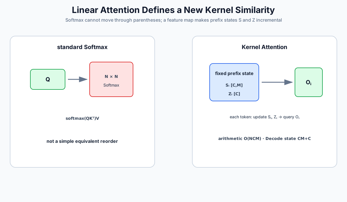
24.4 Linear Attention is not Softmax with different parentheses
Without Softmax, associativity gives:
The left order creates an intermediate; the right creates a intermediate. Standard Attention, however, is:
Softmax normalizes each Query's complete row and cannot simply pass through the parentheses. Kernelized Linear Attention instead chooses a nonnegative feature map and defines a different similarity:
For causal Attention, maintain two prefix states:
Then:
One concrete feature map from the paper is :
import torch
import torch.nn.functional as F


def phi(x):
    return F.elu(x) + 1.0


def causal_kernel_attention(q, k, v):
    """One head: q/k [N,C], v [N,M]."""
    state = q.new_zeros(q.size(1), v.size(1))
    normalizer = q.new_zeros(q.size(1))
    outputs = []
    for q_t, k_t, v_t in zip(phi(q), phi(k), v):
        state = state + torch.outer(k_t, v_t)
        normalizer = normalizer + k_t
        outputs.append((q_t @ state) / (q_t @ normalizer).clamp_min(1e-12))
    return torch.stack(outputs)
With feature dimension and Value dimension , the main cost is . Streaming Decode holds state, fixed with respect to history length. Whether this beats Full Attention depends on , parallelism, and kernels. Most importantly, the code is exact for this Kernel Attention; it is not an error-free rearrangement of standard Softmax Attention.
The chapter's executable tests compare the streaming prefix-state implementation with an explicitly constructed lower-triangular Kernel Attention. Outputs and gradients match in float32 and float64.
24.5 Infini-attention: cross-segment state is what stays fixed
Infini-attention divides input into fixed-length segments. Every layer and Head does two jobs:
- exact causal scaled dot-product Attention inside the current segment for fine local detail;
- retrieval from the previous segment's compressed state, followed by a state update after the current segment is processed.
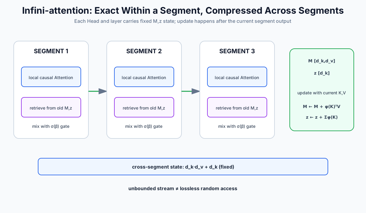
For one Head, the state is not merely a d_model × d_model matrix. It is:
M: [d_key, d_value]
z: [d_key]
Retrieve from old state:
After producing the segment output, update with its K and V:
The paper also evaluates a Delta update; we use its direct Linear version here. Local output and retrieved memory output are mixed with one learned scalar per Head:
import torch
import torch.nn.functional as F


def phi(x):
    return F.elu(x) + 1.0


def retrieve_memory(q, memory, normalizer):
    q_features = phi(q)
    return (q_features @ memory) / (
        q_features @ normalizer
    ).unsqueeze(-1).clamp_min(1e-12)


def infini_segment(q, k, v, memory, normalizer, gate_logit):
    """One head and one segment; q/k [N,D_k], v [N,D_v]."""
    memory_output = retrieve_memory(q, memory, normalizer)
    local_output = F.scaled_dot_product_attention(
        q[None, None], k[None, None], v[None, None],
        is_causal=True, dropout_p=0.0,
    )[0, 0]
    gate = torch.sigmoid(gate_logit)
    output = gate * memory_output + (1.0 - gate) * local_output

    k_features = phi(k)
    next_memory = memory + k_features.T @ v
    next_normalizer = normalizer + k_features.sum(dim=0)
    return output, next_memory, next_normalizer
Order matters: the current segment first reads and writes only after producing its output. The memory branch therefore cannot reveal a future position from the current segment; local causal Attention handles that segment.
24.5.1 What “infinite” means
Per layer and per Head, cross-segment state contains numbers regardless of the number of processed segments. For fixed segment length and total length :
- local Attention costs roughly in total, not total computation;
- compressed state is with respect to ;
- temporary local-Attention memory still depends on and the kernel.
“Infinite” means that a stream need not have a preset total number of segments while the recurrent state remains bounded. It does not mean lossless, random access to every historical token. Many K/V bindings accumulate in one matrix, so interference and information loss are part of the compression.
24.5.2 Paper results are not Gemini 1.5 architecture disclosure
After the corresponding training, the Infini-attention paper reports a 1B model on a 1M-length passkey-retrieval task and an 8B model on 500K-length book summarization. Those are paper-specific models, tasks, and training conditions.
The Gemini 1.5 technical report appeared in March 2024; the first Infini-attention arXiv version appeared in April 2024. Neither public report states that Gemini 1.5 uses Infini-attention. Equating them because both address long context is speculation, not an architecture fact.
24.6 Put each method back on the right axis
| Method | What changes | Main term for total length | Exact historical retention? | Important condition |
|---|---|---|---|---|
| Full + FlashAttention | Kernel / I/O | arithmetic | Yes, inside the window | Full score matrix is not written to HBM |
| Sliding Window | Connection graph | Outside-window influence is indirect | Fixed and a kernel that exploits structure | |
| Longformer / BigBird | Local, global, random graph | Only allowed edges are exact | Original claims have task and graph boundaries | |
| Kernel Linear Attention | Similarity and order | Compressed into | Not a simple Softmax equivalence | |
| Infini-attention | Recurrent cross-segment state | Linear in for fixed segment | Cross-segment history is compressed | Requires adapted training; local Attention remains |
Some combinations are mathematically compatible, but that does not mean every framework provides an efficient fused kernel. FlashAttention, GQA, block-sparse masks, Rolling Cache, and compressed memory operate at different layers. Every added mechanism needs fresh validation of correctness, quality, peak memory, and measured throughput.
24.7 Chapter summary
- Full Attention has quadratic pairwise work. Materialized score storage and linear KV Cache are separate bills.
- Sparse Attention saves work only with a kernel that skips empty blocks; a dense matrix plus mask merely produces a sparse result.
- Longformer and BigBird are linear only when window, global, and random counts stay fixed. Theoretical expressivity is not a quality guarantee on arbitrary tasks.
- Linear Attention defines a new Kernel similarity through a feature map. It is not standard Softmax Attention with different parentheses.
- Infini-attention keeps bounded with respect to total history, but total computation grows with processed segments and cross-segment history is lossy.
- Public evidence does not establish that Gemini 1.5 uses Infini-attention.
References
- Longformer: The Long-Document Transformer (Beltagy et al., 2020)
- Big Bird: Transformers for Longer Sequences (Zaheer et al., 2020)
- Transformers are RNNs: Fast Autoregressive Transformers with Linear Attention (Katharopoulos et al., 2020)
- Leave No Context Behind: Efficient Infinite Context Transformers with Infini-attention (Munkhdalai et al., 2024)
- Mistral 7B (Jiang et al., 2023)
- Gemini 1.5: Unlocking multimodal understanding across millions of tokens of context (Gemini Team, 2024)
- PyTorch FlexAttention documentation
Next chapter
This chapter quietly assumed that the model knows relative positions: a window must slide in a direction, causality needs an order, and segments need a position scheme. Chapter 25 returns to that foundation and follows positional encoding from absolute positions to relative distance, rotation, and linear bias.