One-sentence summary: Matrix multiplication is more than rows times columns: it applies linear maps and batches dot products, while the dot product itself has angle and projection interpretations that make Attention easier to see.

8.1 Why Learn This Before Attention?

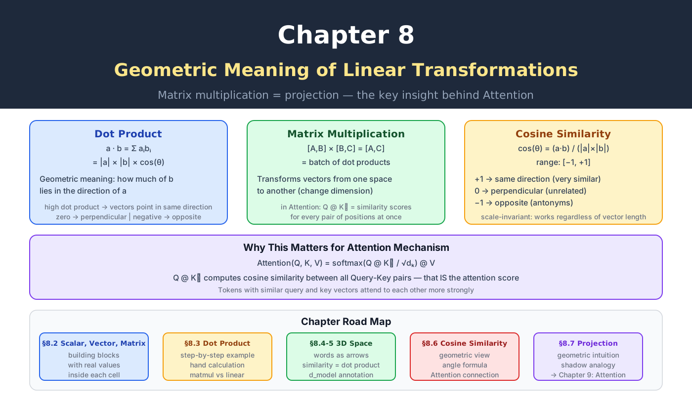
Linear maps, batched dot products, cosine similarity, and projection as preparation for Attention

Attention is full of matrix multiplication. If you only think about it as rows times columns, the QKV mechanics will feel like symbol-pushing. If you see it as geometry, the architecture clicks.

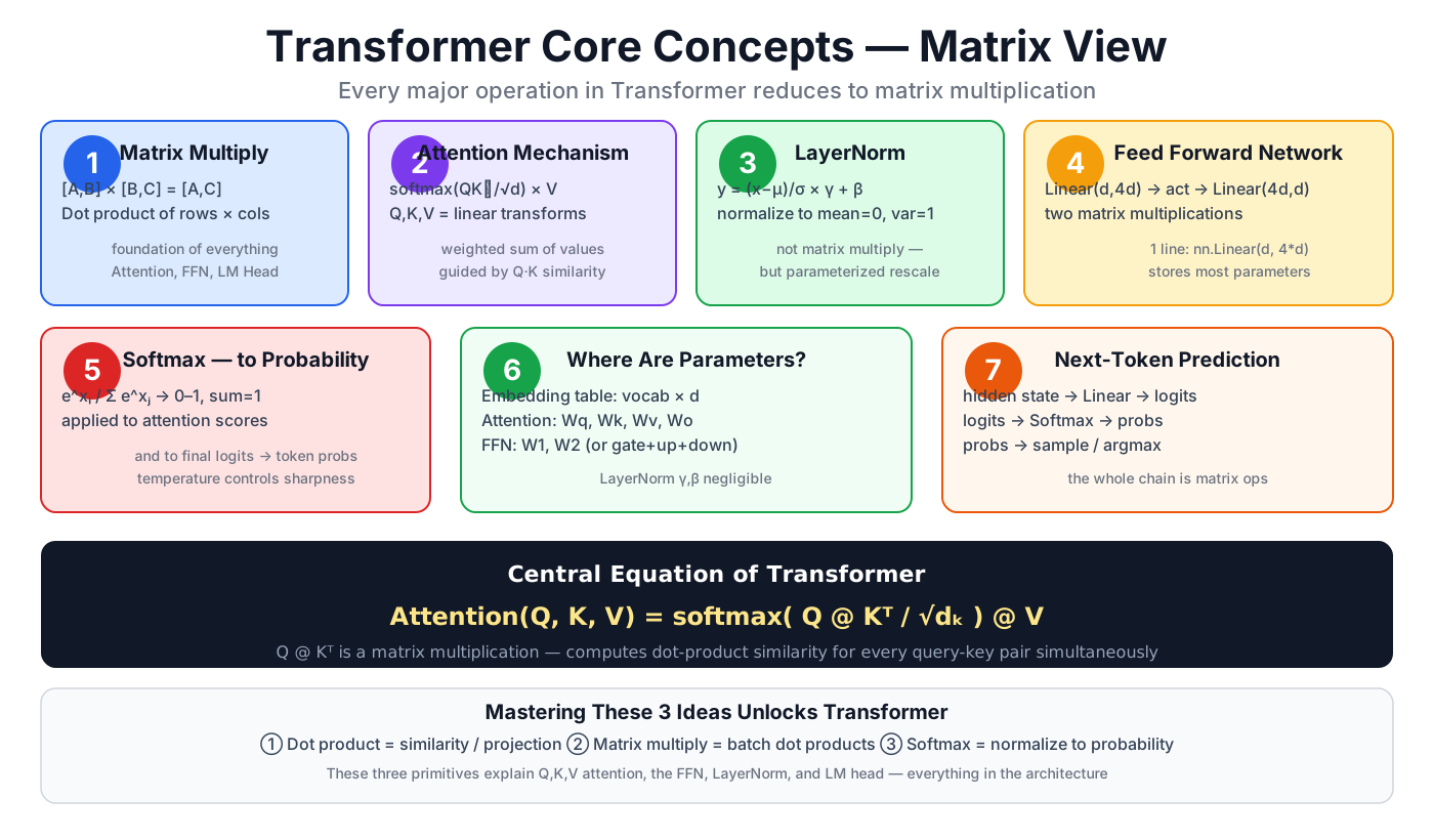
Transformer tensor operations, separating learned matrix projections from LayerNorm and Softmax

Here is a map of where matrix multiplication appears in the Transformer:

Embedding lookup (normally indexing; equivalently one-hot vector × embedding table)
Q, K, V projection matrices in Attention
FFN expand and contract layers
Final vocabulary projection (LM Head)

Matrix multiplication is everywhere in the learned projections. LayerNorm and Softmax are different operations, but understanding matrix multiplication geometrically is still the highest-leverage preparation for Chapter 9.

8.2 Scalars, Vectors, and Matrices

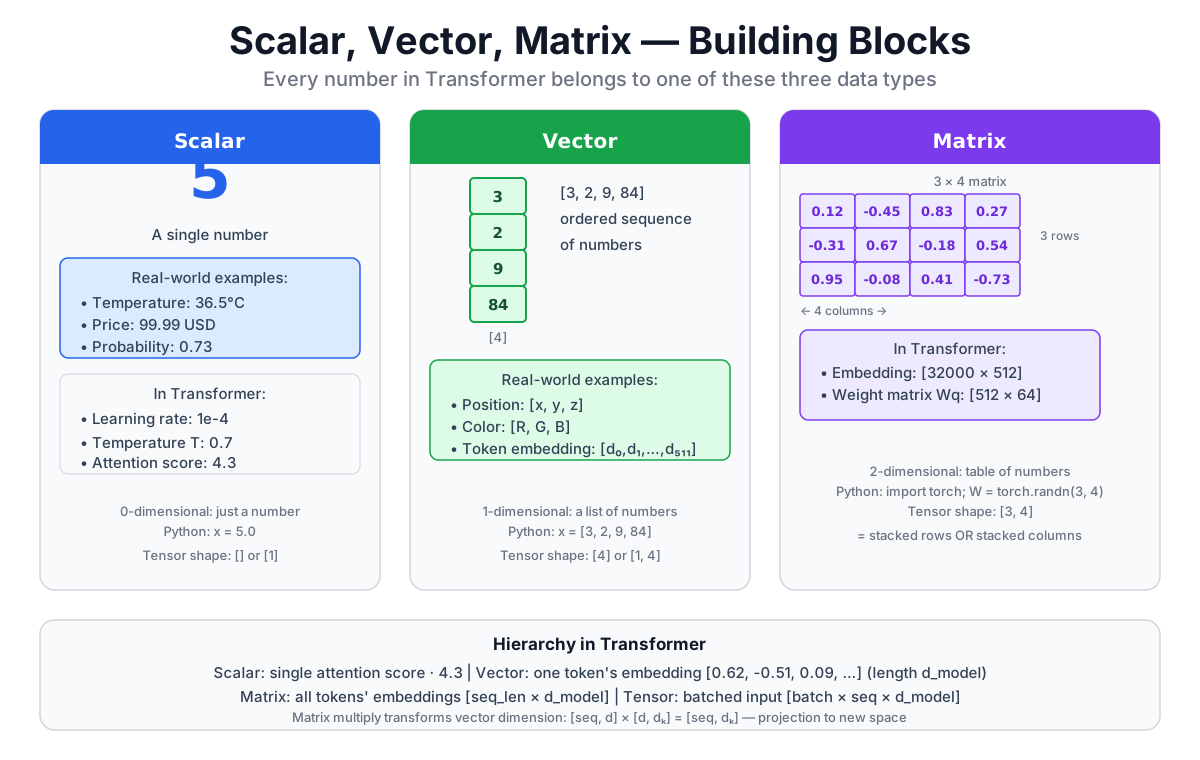
Scalar is one number; vector is an ordered list; matrix is a 2D table

Before going further, let's fix the vocabulary.

8.2.1 Scalar

A scalar is a single number.

Temperature, learning rate, attention score at one position — these are all scalars.

8.2.2 Vector

A vector is an ordered list of numbers.

[3, 2, 9, 84]

Vectors can represent almost anything: a 3D position [x, y, z], an RGB color [255, 128, 0], or a token's semantic representation in a 4096-dimensional space. The key property is that the order matters.

8.2.3 Matrix

A matrix is a 2D table of numbers.

3 × 4 matrix:
┌─────────────────┐
│  □  □  □  □  │
│  □  □  □  □  │
│  □  □  □  □  │
└─────────────────┘

You can think of a matrix as a stack of row vectors, or equivalently as a collection of column vectors.

8.2.4 In the Transformer

Object	Example
Scalar	learning rate, temperature, one attention score
Vector	one token's embedding (shape: `[d_model]`)
Matrix	all token embeddings at once (shape: `[seq_len, d_model]`) or a weight matrix `[d_model, d_model]`

The token representation flowing through the Transformer is a matrix of shape [seq_len, d_model] — one row per token, one column per feature dimension.

8.3 Matrix Multiplication: The Computation

8.3.1 Dimension Rule

The dimension rule for matrix multiplication:

[A, B] × [B, C] = [A, C]

The inner dimensions must match (both B). The output shape is the two outer dimensions.

8.3.2 Worked Example

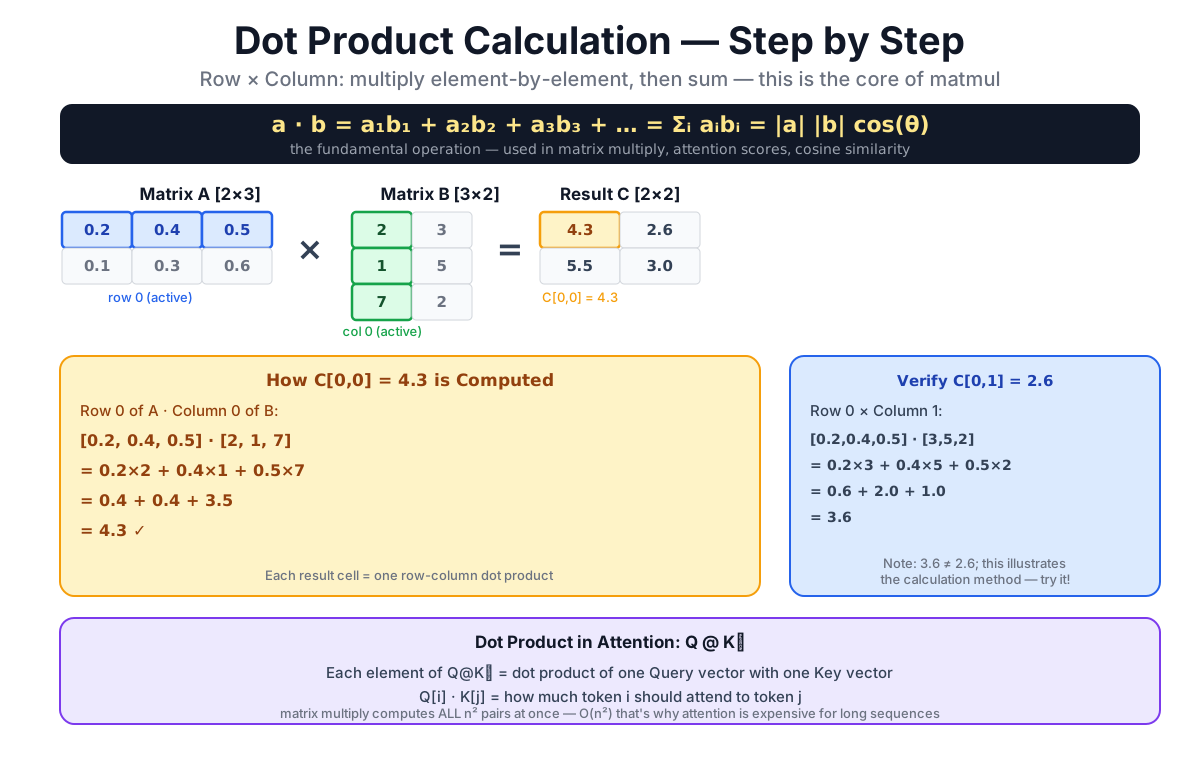
Dot product calculation: first row times first column gives the top-left element of the result

Let's compute a [4, 3] × [3, 4] multiplication. The result is [4, 4].

For the first element of the result (row 0, column 0):

row 0 of left matrix: [0.2, 0.4, 0.5]
col 0 of right matrix: [2, 1, 7]

dot product: 0.2×2 + 0.4×1 + 0.5×7
           = 0.4 + 0.4 + 3.5
           = 4.3

The fundamental operation is the dot product: multiply corresponding elements and sum.

In Python/NumPy/PyTorch:

C = A @ B  # @ is the matrix multiplication operator

8.3.3 Why "Dot Product"?

The name comes from the mathematical notation A · B. For two vectors of the same length:

A · B = a₁b₁ + a₂b₂ + a₃b₃ + ... + aₙbₙ

A matrix multiply is just many dot products organized into a grid.

8.4 Two Ways to Think About the Same Operation

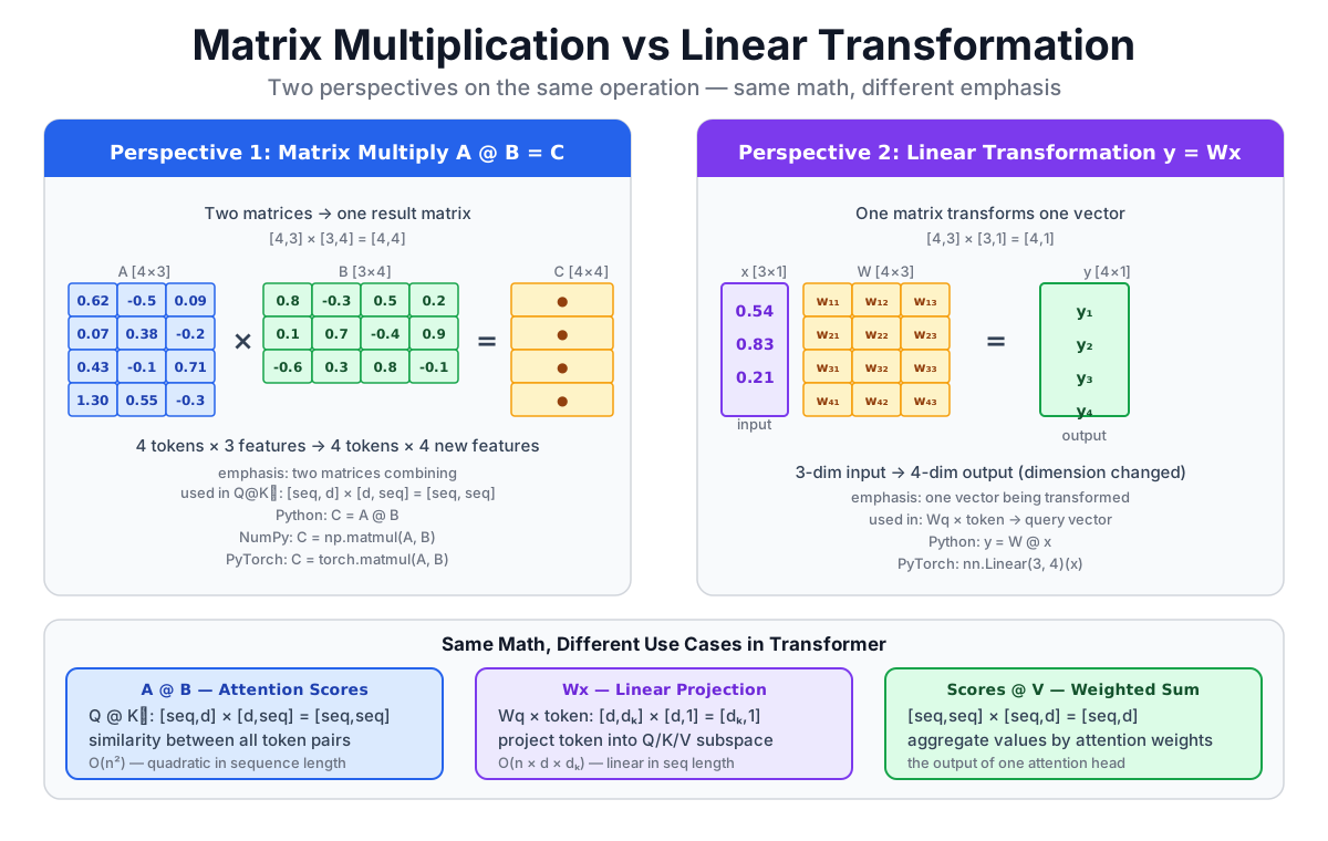
Two views of matrix multiplication: raw dot products vs linear transformation of a vector

The same operation has two useful frames.

8.4.1 Frame One: Dot Product (Matrix × Matrix)

[4, 3] × [3, 4] = [4, 4]

Two matrices multiply. Each element of the output is a dot product between a row of the left matrix and a column of the right matrix.

This frame is useful when both operands contain vectors — for example, computing all pairwise dot-product scores.

8.4.2 Frame Two: Linear Transformation (Matrix × Vector)

[4, 3] × [3, 1] = [4, 1]

A weight matrix transforms a single vector: input dimension changes from 3 to 4.

This frame is useful when one operand is data and the other is a learned weight matrix. The weight matrix defines a learned transformation of the vector space.

8.4.3 Linear Transformation Intuition

"Linear transformation" sounds technical. The geometric idea is simple:

A weight matrix maps a vector from one space to another — possibly changing its dimension, rotating it, stretching it, shearing it, or projecting it down.

In the Transformer:

An embedding layer normally indexes a row of the embedding table. If the token ID is represented as a one-hot vector, the same lookup is equivalent to multiplying by that table.
The Q, K, V weight matrices move d_model vectors into a different d_model (or d_key) space, emphasizing different aspects.
The FFN expand layer moves vectors from d_model into 4 × d_model space.

Linear transformations are everywhere because vectors in different "views" of the same data are what the model learns to compare.

8.5 Geometric Meaning: Vector Space

Now for the part that makes Attention click.

8.5.1 Word Vectors in 3D

Four hand-built 3D toy vectors and their corrected pairwise dot-product matrix

Suppose we hand-build a tiny 3D toy space with four vectors:

cat  = [7, 7, 6]
fish = [6, 4, 5]
love = [-4, -2, 1]
eat  = [6, 5, 7]

Plot these as arrows from the origin in 3D space:

cat and fish point in roughly the same direction.
love points in a very different direction.

These numbers were chosen to make the geometry easy to draw; they are not measurements from a real model. Real token representations change with context and layer. Directional structure can carry semantic information, but this toy picture does not prove that two words must be close in a trained model.

8.5.2 Matrix Multiplication Batches Dot Products

Stack n vectors as the rows of X, and one matrix multiplication computes every pairwise dot product:

X [n, d] @ X.T [d, n] = S [n, n]

Each S[i,j] is the dot product between vectors i and j. With the toy values above, cat · fish = 100, love · fish = -27, and eat · fish = 91.

A dot product depends on both direction and magnitude. It can serve as a learned compatibility score, but it is not pure cosine similarity. This is why matrix multiplication appears inside Attention: QKᵀ computes all Query-Key compatibility scores in one operation.

8.5.3 The `d_model` Dimension

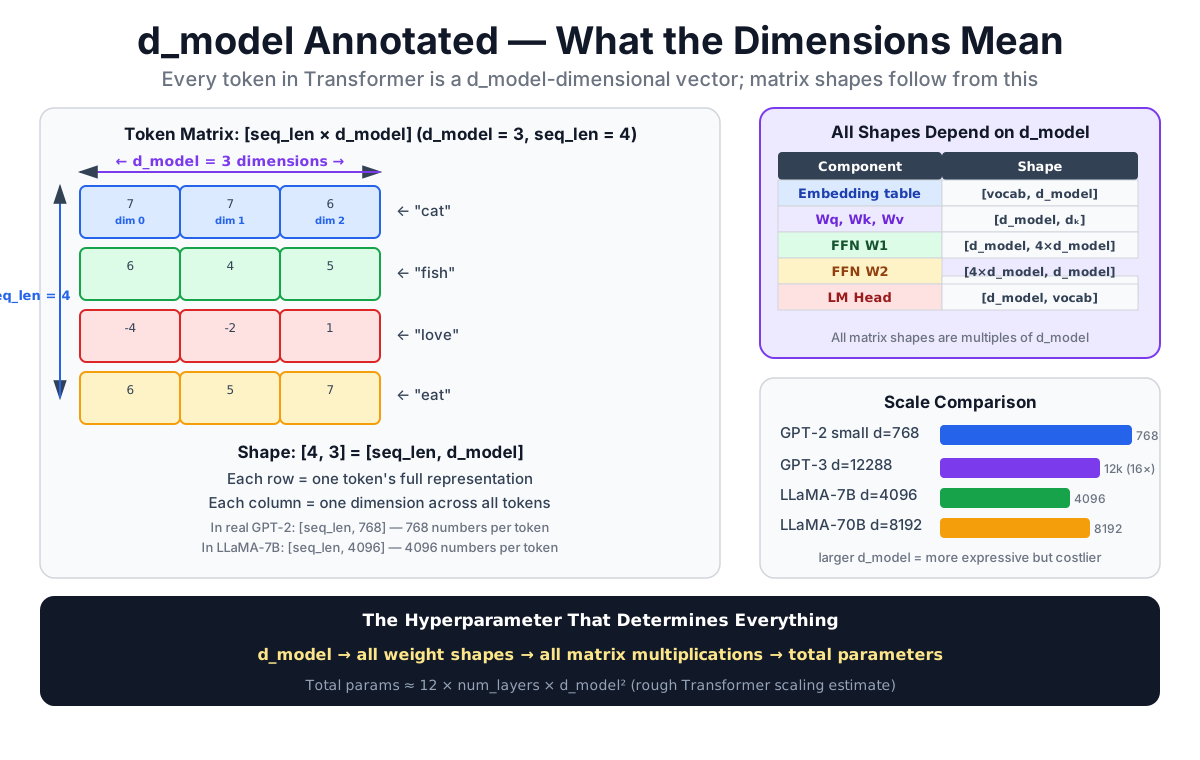
d_model annotated on the token matrix: each column is one feature dimension

d_model is the number of dimensions in each token's representation:

Model	d_model
GPT-2 Small	768
GPT-2 Large	1,280
GPT-3	12,288
Llama 2 7B	4,096

More dimensions generally provide more representational capacity — more directions available to encode distinctions — but do not guarantee a better model. They also mean larger weight matrices and more computation.

8.6 Dot Product and Cosine Similarity

8.6.1 The Angle Between Vectors

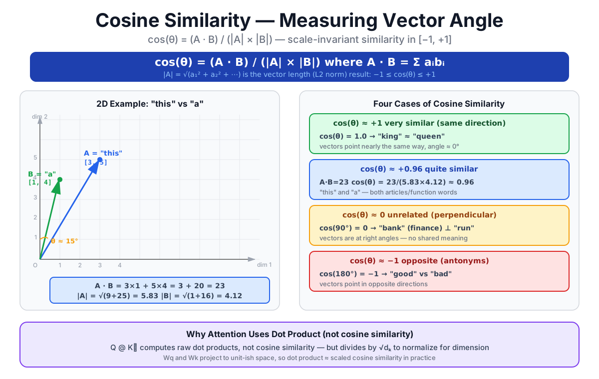
Cosine similarity: the dot product relates to the angle between two vectors

The dot product relates to the angle between vectors through a formula:

\cos(\theta) = \frac{A \cdot B}{|A| \times |B|}

Rearranging:

A \cdot B = |A| \times |B| \times \cos(\theta)

Where:

|A| is the length (magnitude) of vector A.
|B| is the length of vector B.
θ is the angle between them.

8.6.2 Geometric Intuitions

Situation	cos(θ)	dot product	Interpretation
Same direction	1	positive (`	A
90° apart	0	0	geometrically orthogonal
Opposite directions	-1	negative (`-	A

This gives us a clean geometric reading of the dot product: it combines directional alignment with vector magnitude. Cosine similarity removes the magnitude term and keeps only the angle. These geometric labels are not automatic semantic labels: orthogonal need not mean “unrelated,” and anti-aligned need not mean “antonyms.”

8.6.3 A Concrete Example

A = [3, 5]
B = [1, 4]

Compute:

A · B = 3×1 + 5×4 = 3 + 20 = 23
|A| = √(9 + 25) = √34 ≈ 5.83
|B| = √(1 + 16) = √17 ≈ 4.12

cos(θ) = 23 / (5.83 × 4.12) ≈ 23 / 24.0 ≈ 0.96

These two toy vectors have a cosine similarity of 0.96 — nearly parallel. They are not measured embeddings for any words.

8.6.4 This Is the Core of Attention

In Attention:

A Query vector asks: "What am I looking for?"
A Key vector says: "Here is what I contain."
Their dot product provides a learned compatibility score between the Query and Key.

For one Query, a relatively high score on an unmasked Key usually becomes a relatively high attention weight after scaling and Softmax.

Attention uses dot products to score learned Query-Key compatibility. It does not normalize Q and K by their lengths, so the score is not cosine similarity.

8.7 Projection: A Second Geometric View

8.7.1 What Projection Means

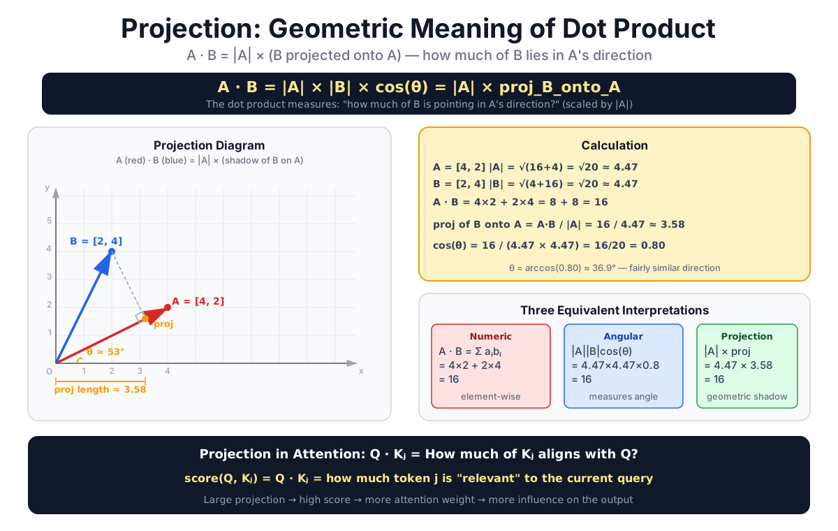
Projection: how much of vector B lies in the direction of vector A

The dot product has a second geometric interpretation: projection.

A · B = |A| × (signed length of B projected onto A's direction)

Or equivalently:

A · B = |B| × (signed length of A projected onto B's direction)

Projection asks: how much of one vector's "content" lies in the direction of another?

8.7.2 The Projection Picture

In a 2D sketch:

Draw vector A (red arrow).
Draw vector B (blue arrow).
Drop a perpendicular from the tip of B onto the line defined by A.
The length from the origin to that foot is the projection of B onto A.

The dot product equals |A| times that signed scalar projection. The projection vector itself is:

proj_A(B) = (A · B / |A|²) A

8.7.3 Why This Matters for Language

In a trained model, Q and K projections are learned. Some directions can become useful for a task, but there is usually no single coordinate axis neatly labeled “royalty” or “abstractness.” Projection is a geometric intuition for the formula, not a license to assign a human concept to one neuron or dimension.

8.8 Connecting Back to Attention

8.8.1 The Attention Formula Preview

The core of Attention (details in Chapter 9):

\text{Attention}(Q, K, V) = \text{softmax}\!\left(\frac{QK^T}{\sqrt{d_k}} + M\right) V

The term QK^T computes dot products between every Query and Key simultaneously. The result is a matrix of compatibility scores. M is a causal or padding mask: allowed positions add zero, blocked positions add negative infinity before Softmax.

8.8.2 Reading Q, K, V Geometrically

Q = X W_Q
K = X W_K
V = X W_V

Read this as: take the input X and view it through three learned geometric lenses. Each matrix W_Q, W_K, W_V maps the same input representation into vectors with a different job:

W_Q projects into a "what am I looking for" space.
W_K projects into a "what do I advertise" space.
W_V projects into a "what information do I contribute" space.

The dot product between Q and K vectors gives a learned compatibility score. After division by √d_k, masking, and Softmax, a larger relative score gives that token's Value more weight in the output.

8.8.3 Summary of the Geometric Reading

Math	Geometric meaning	Role in Attention
`A · B`	magnitude-aware alignment / projection	scores Query-Key compatibility
matrix multiply `AB`	batch dot products	computes all pairwise scores at once
Softmax	exponential normalization	converts each row of scores into weights summing to 1

8.9 Chapter Summary

8.9.1 Key Concepts

Concept	Meaning
Scalar	a single number
Vector	an ordered list of numbers; represents a point or direction
Matrix	a 2D table; represents a transformation or a batch of vectors
Dot product	element-wise multiply and sum; combines alignment and magnitude
Linear transformation	using a weight matrix to rotate/stretch/project a vector
Cosine similarity	dot product normalized by vector lengths; pure angle measure
Projection	how much of one vector lies in the direction of another

8.9.2 Key Formulas

Dot product:

A · B = a₁b₁ + a₂b₂ + ... + aₙbₙ

Cosine similarity:

\cos(\theta) = \frac{A \cdot B}{|A| \times |B|}

Projection of B onto A:

A · B = |A| × (B projected onto A)

Matrix multiply dimension rule:

[A, B] × [B, C] = [A, C]

8.9.3 Core Takeaway

Do not collapse two ideas into one: matrix multiplication can apply a general linear map or batch many dot products; the dot product is the operation with angle and projection interpretations. Attention uses it to score every Query-Key pair, then scales, masks, and normalizes those scores into weights.

Chapter Checklist

After this chapter, you should be able to:

State the dimension rule for matrix multiplication and compute a small example by hand.
Explain the dot product as a measurement of vector alignment.
Explain projection in plain English: how much of one vector lies in another's direction.
Explain why matrix multiply is the right tool for computing all pairwise Query-Key compatibility scores.
Connect the dot product to the Query-Key matching inside Attention.

See You in the Next Chapter

That is the geometry. If you can draw two arrows, explain why their dot product depends on angle and length, and trace a relative score through scaling, masking, and Softmax, you are ready for Chapter 9.

Chapter 9 closes the loop: we put the geometric intuition together with the actual Attention formula, look at what attention heatmaps reveal, and answer the question of why dot product specifically — rather than some other similarity measure — became the standard choice.