One-sentence summary: A neural network layer is a learned function that transforms vectors through matrix multiplication and nonlinearity — and for understanding the Transformer, treating it as a shape-changing black box gets you most of the way there.
7.1 You Do Not Need to Be a Neural Network Expert
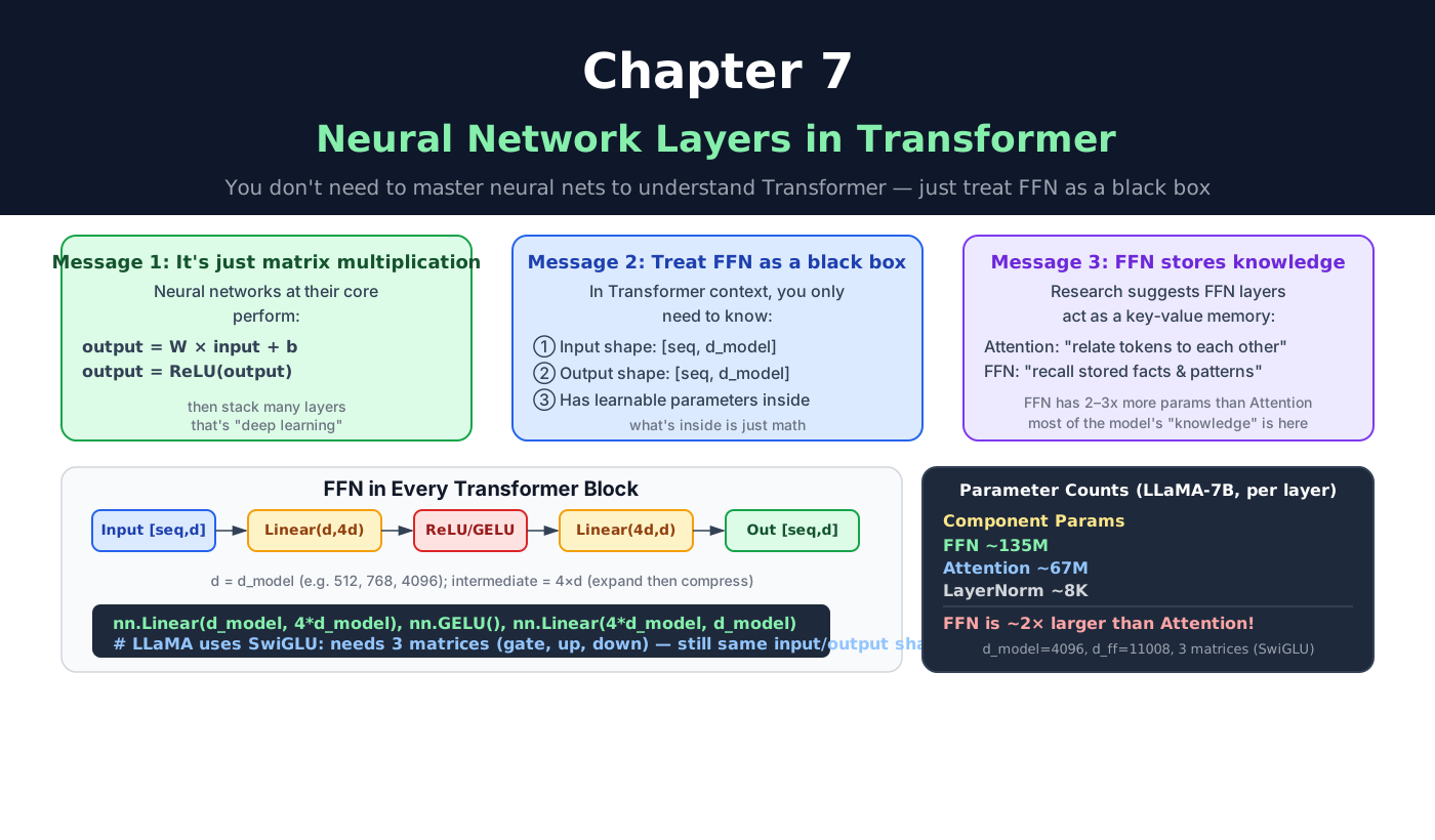
Let me say this plainly before going any further: you do not need to deeply understand neural networks to understand the Transformer.
Inside each Transformer block, the Feed Forward Network (FFN) is a neural network layer. But its role in the architecture is simple: it receives a vector, transforms it, and returns a vector of the same size. For the purposes of understanding how the whole Transformer works, you can treat it as a learned function with a known shape.
What you do need to know:
- What shape goes in.
- What shape comes out.
- Where the learnable parameters live.
If you want the deeper picture, this chapter has it. But the goal is to give you a working mental model, not to turn you into a backprop engineer.
7.2 The Biological Inspiration (and Why It Only Goes So Far)
7.2.1 Biological Neural Networks
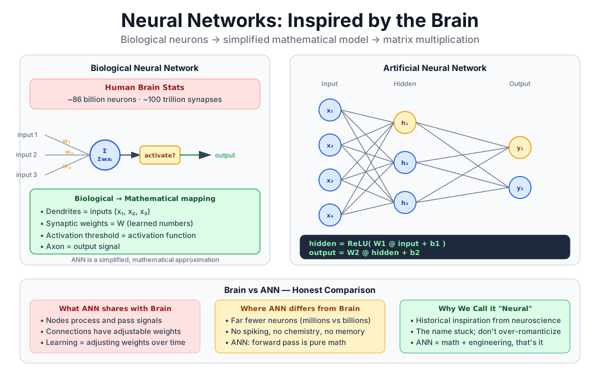
At the level of rough counts, an adult human brain has:
- about 86 billion neurons: an experimental estimate, not a round-number analogy
- on the order of 10¹⁴ synapses: roughly 100 trillion connections, with substantial estimation uncertainty
A neuron receives electrical signals from upstream neurons. When the total incoming signal crosses a threshold, the neuron "fires" and sends a signal downstream.
7.2.2 Artificial Neural Networks
Artificial neural networks borrow the vocabulary but not the full biology:
- Node: models a neuron
- Weight: models a synapse strength
- Activation function: applies a nonlinear transformation to the weighted result; it need not be a hard threshold
The important disclaimer: an artificial neural network is a mathematical model, not a simulation of the brain. It borrows the name and the rough metaphor. The actual computation is matrix multiplication plus a nonlinear function.
Do not let the "neural" branding make this feel mystical. It is linear algebra with a twist.
7.3 What Neural Networks Learn to Do
7.3.1 Automatic Feature Discovery
The compelling property of neural networks is that they can learn useful representations without having every feature rule hand-written.
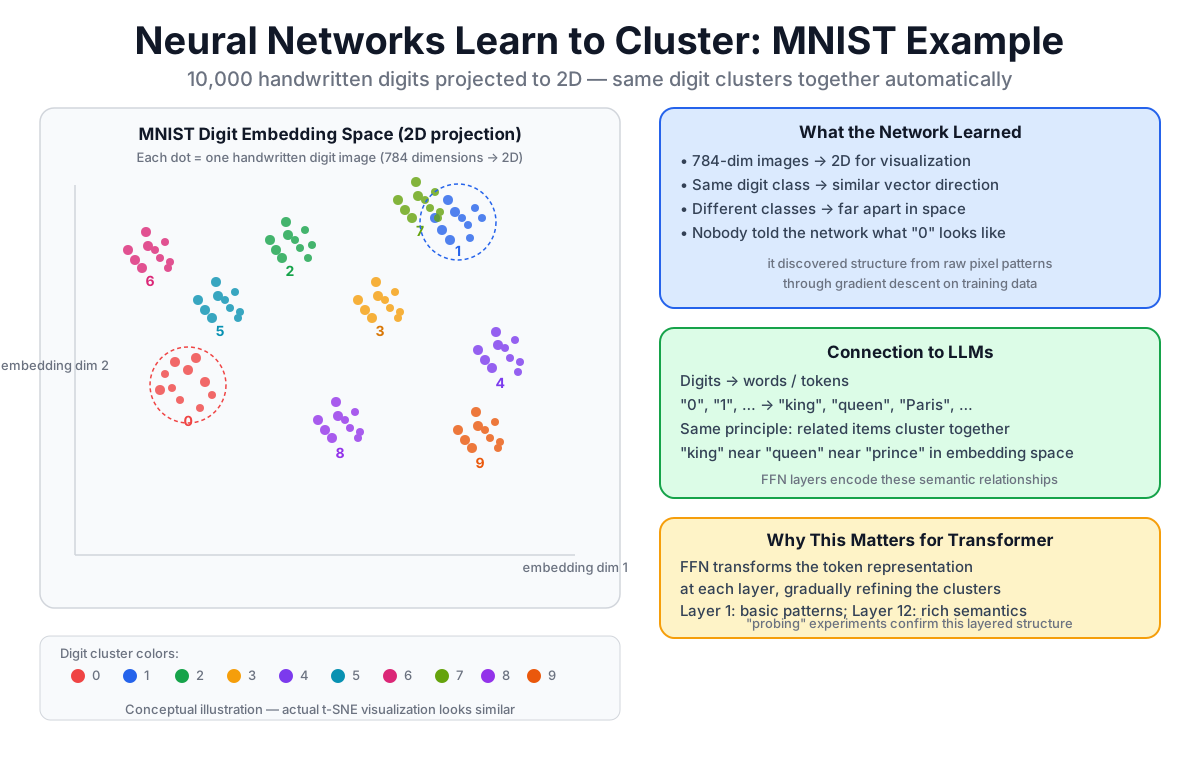
A classic demonstration is to train a digit classifier on MNIST. Each image is 28×28 pixels = 784 dimensions. Project a hidden representation down to 2D with t-SNE, UMAP, or another visualization method, and examples of the same class often appear near one another. The exact map depends on the model, layer, and projection method; the illustration here is conceptual, not measured output from a particular run.
The labels do tell a classifier which examples are threes. What nobody hand-codes is a pixel rule for what a "3" must look like. The network learns a useful representation from the training signal.
7.3.2 The Language Parallel
The same principle applies to language. Given enough training text:
- The model learns which words tend to co-occur.
- It learns grammatical structure from distribution patterns.
- It may learn that “thereminist” and “inventor” can occupy similar syntactic slots.
After training, internal token representations can exhibit semantic and syntactic structure. But “these two phrases are always nearby” is not a fixed rule: representations change with context, layer, and model.
7.4 The Basic Structure of a Neural Network
7.4.1 Three Layers
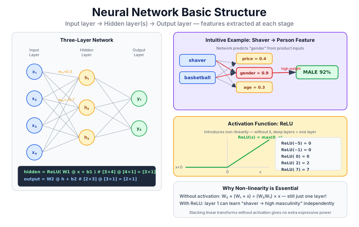
A common teaching diagram has three parts:
- Input layer: receives the raw data — in our case, a token vector.
- Hidden layer: performs an intermediate transformation.
- Output layer: returns the result.
"Hidden" just means the layer is not directly observed as input or output. A network can have no hidden layer or many hidden layers, and both hidden and output transformations can contain learnable weights.
7.4.2 An Example with Concrete Features
Suppose the input is a vector that represents a product listing. The hidden layer might learn internal features like:
- waterproofing
- warmth
- weight
From those features, the output layer might predict a category such as rainwear or winter clothing.
The network learns:
- Which input dimensions to combine for each feature.
- Which feature combinations predict which labels.
Nobody handcrafted those intermediate features. The network discovered them by minimizing prediction error on the training data.
7.5 The Mathematical Core: Matrix Multiplication
7.5.1 One Dense Layer = One Affine Transform
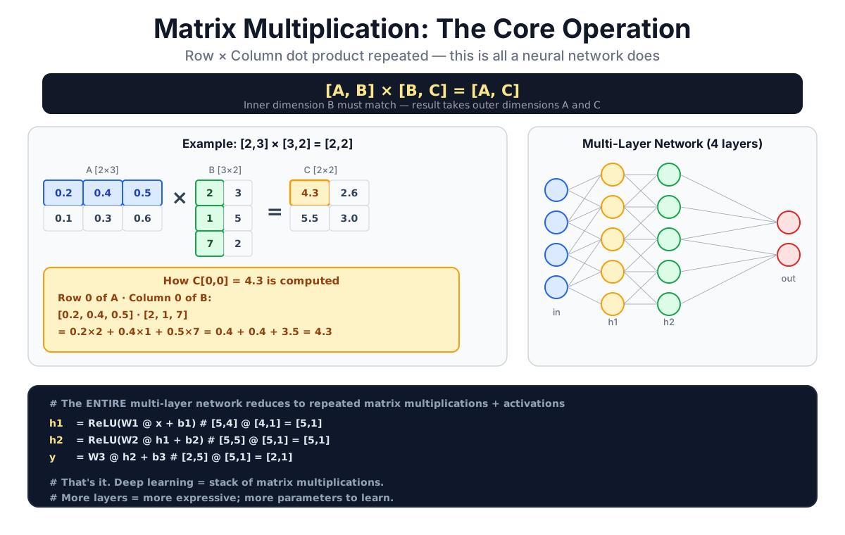
The core computation of a single dense (fully connected) layer:
y = xW + bWhere:
xis the input vector.Wis the weight matrix — the learnable parameters.bis the bias vector — also learnable.yis the output vector.
Concretely, using row-vector notation for a 2D input and 2D output:
input vector × weight matrix = output vector

[0.54, 0.84] × [w₁ w₃] + [b₁, b₂] = [0.91, 0.90]
               [w₂ w₄]
The shapes are [1, 2] @ [2, 2] = [1, 2]. The output element at position i is the dot product of the input with the i-th column of W. Column-vector notation is also valid, but then the order is W @ x; [2,1] @ [2,2] would not be valid.
7.5.2 Multiple Layers
When you stack multiple layers:
layer 1 -> layer 2 -> layer 3 -> layer 4Each learned arrow is an affine transform, with nonlinearities between hidden layers. "Deep learning" broadly refers to learning with multi-layer neural networks, not to matrix multiplication alone.
In the figure, the connections between nodes represent the weights. Every connection is one element of a weight matrix. More layers = more matrices = more learnable parameters.
7.5.3 Why This Matters for Parameter Counts
When someone says "GPT-3 has 175 billion parameters," most of those parameters are numbers inside weight matrices like these. They are not stored in a separate knowledge base. They are the learned values of W in every layer.
7.6 Activation Functions: The Nonlinear Ingredient
7.6.1 Why Nonlinearity Matters
If you stack only linear layers:
y₂ = (x W₁) W₂ = x (W₁ W₂) = x W₃Multiple matrix multiplications collapse into a single matrix multiply. No matter how many layers you add, the whole stack is equivalent to one layer. You cannot represent complex patterns this way.
Activation functions insert nonlinearity between layers, breaking this collapse.
7.6.2 ReLU
The simplest widely-used activation is ReLU (Rectified Linear Unit):
ReLU(x) = max(0, x)Positive values pass through unchanged. Negative values become zero.
import torch
import torch.nn as nn

x = torch.tensor([-2.0, -1.0, 0.0, 1.0, 2.0])
print(nn.functional.relu(x))  # tensor([0., 0., 0., 1., 2.])
7.6.3 GELU and SwiGLU
Modern LLMs use other choices, including gated FFNs:
- GELU (Gaussian Error Linear Unit): used in GPT-2, BERT, many others. Smoother than ReLU around zero.
- SwiGLU: used in Llama and many later models. It gates one projection with a SiLU-activated second projection, then applies a third projection back to
d_model.
For understanding the architecture, you do not need to memorize these. The important point is that the FFN inserts nonlinearity between projections. Not every Linear in a model is followed by an activation.
7.7 PyTorch Implementation
7.7.1 A Simple Network
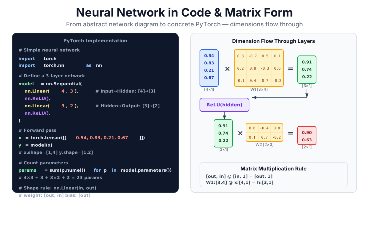
import torch.nn as nn

model = nn.Sequential(
    nn.Linear(2, 3),   # input layer:  2-dim → 3-dim
    nn.ReLU(),         # activation function
    nn.Linear(3, 1),   # output layer: 3-dim → 1-dim
)
Seven lines (including the blank line and comments). That is a complete feedforward network.
Conceptually, row-vector notation often uses a matrix shaped [in_features, out_features]. PyTorch stores nn.Linear(in_features, out_features).weight as [out_features, in_features] and computes x @ weight.T + bias; the bias is shaped [out_features].
7.7.2 Dimension Changes
The shape of data as it passes through:
input (1, 2) @ weight (2, 3) = hidden (1, 3) @ weight (3, 1) = output (1, 1)Matrix multiplication rule: (a, b) @ (b, c) = (a, c). The inner dimensions must match. The outer dimensions are the result shape.
Understanding dimension changes is the key to reading Transformer code.
7.8 The FFN in the Transformer Block
7.8.1 The Expand-Then-Contract Pattern
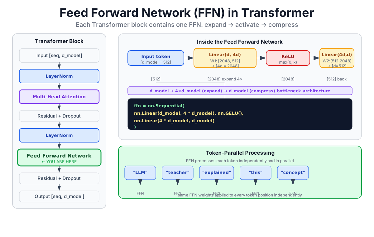
In the original Transformer and GPT-2-style blocks, the Feed Forward Network (FFN) commonly uses this shape:
[d_model] → [4 × d_model] → [d_model]The vector expands to four times its width, passes through a nonlinear activation, then contracts back to d_model. Four is a classic configuration, not a universal rule.
ffn = nn.Sequential(
    nn.Linear(d_model, 4 * d_model),   # expand
    nn.GELU(),                          # activation
    nn.Linear(4 * d_model, d_model),   # contract
)
This is the standard FFN for GPT-2-style models. Llama 2 uses a SwiGLU variant with three matrices and d_ff = 11008 for d_model = 4096, but the expand-then-contract idea is the same.
7.8.2 The Full Block Structure
Input
  ↓
Norm (LayerNorm or RMSNorm)
  ↓
Masked Multi-Head Attention
  ↓
Residual connection
  ↓
Norm (LayerNorm or RMSNorm)
  ↓
Feed Forward Network (FFN)    <- this is the neural network layer
  ↓
Residual connection
  ↓
Output
Attention mixes information across positions. The FFN processes each position's representation independently. The two sub-layers have complementary roles:
- Attention asks: which other tokens in the sequence are relevant to this one?
- FFN provides a learned nonlinear transformation of that position's current representation.
7.8.3 Why Each Token Independently?
The FFN applies the same transformation to each token position without mixing across positions. That happens inside Attention. Keeping the operations separate makes the architecture easier to scale and modify.
7.9 Where Are the Parameters?
7.9.1 Every Learnable Weight Matrix
Here is a map of where parameters live in a Transformer:
| Component | Parameters |
|---|---|
| Embedding table | vocab_size × d_model |
| Traditional two-matrix FFN (per block) | about 2 × d_model × d_ff, plus any biases |
| SwiGLU FFN (per block) | about 3 × d_model × d_ff |
| Full MHA Q, K, V, O (per block) | about 4 × d_model²; MQA/GQA use smaller K/V projections |
| One LayerNorm / RMSNorm module | 2 × d_model for LayerNorm with scale and bias; usually d_model for RMSNorm |
| LM Head (final projection) | d_model × vocab_size; sharing with the input embedding is model-specific |
7.9.2 Parameter Counts for a Realistic Model
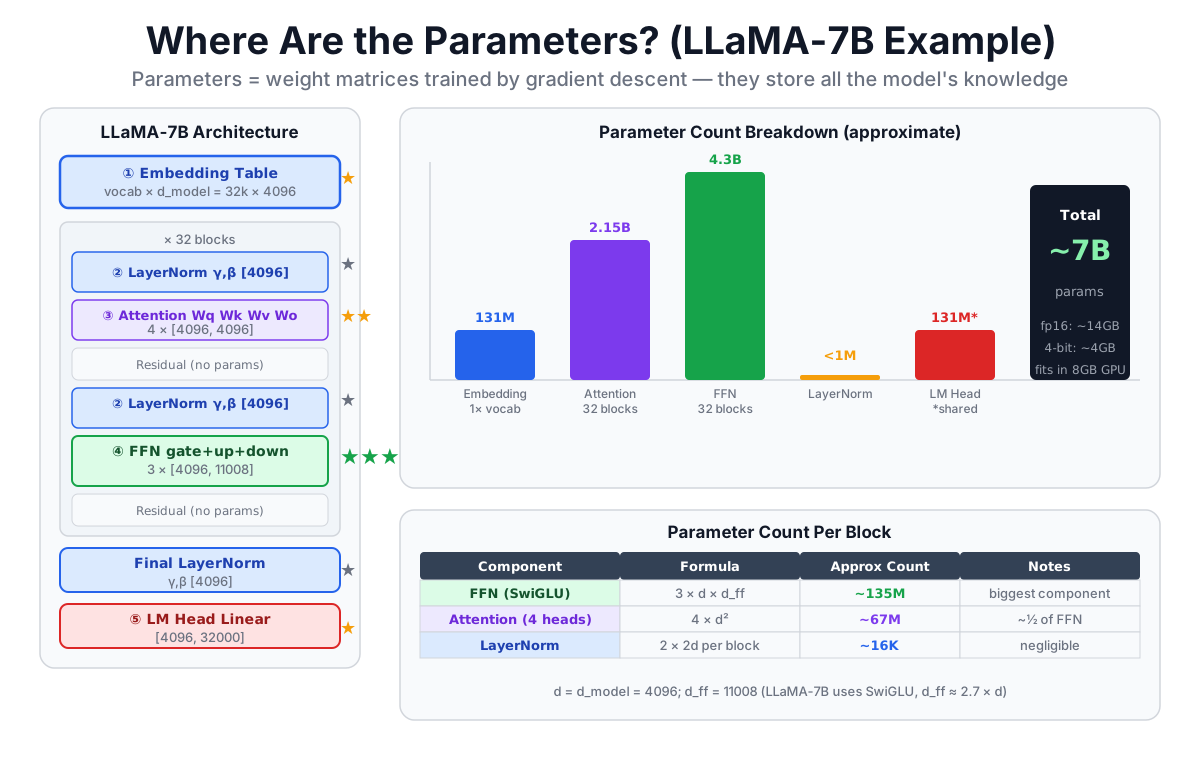
For Llama 2 7B (d_model = 4096, d_ff = 11008, 32 blocks, vocab_size = 32,000), using weight-only counts:
| Component | Parameters |
|---|---|
| Embedding | 32,000 × 4,096 ≈ 131M |
| FFN per layer (SwiGLU, 3 matrices) | 3 × 4,096 × 11,008 ≈ 135M |
| Attention per layer | 4 × 4,096² ≈ 67M |
| RMSNorm per block | two scale vectors: 2 × 4,096 = 8,192 |
| LM Head | 4,096 × 32,000 ≈ 131M, separate from the input embedding |
*Llama 2 uses SwiGLU, which requires gate, up, and down projections rather than the two matrices in a traditional FFN. Its Linear layers do not use bias.
7.9.3 The Surprising Fact About FFN
Many people assume Attention is where most parameters live, because Attention is where the "interesting" computation happens. In this concrete model, however, the FFN has about 135M parameters per block and MHA about 67M: almost exactly twice as many.
Across 32 layers, the FFN accounts for the majority of the parameter budget.
A useful intuition is that Attention routes and mixes information across positions, while the FFN applies a nonlinear transformation at each position. Research has also modeled FFNs as key-value memories and located or edited factual associations through them. That is evidence for an important memory-like role, not proof that knowledge lives in one component: embeddings, Attention, FFNs, and the residual stream all participate in model behavior.
7.10 Chapter Summary
7.10.1 Key Concepts
| Concept | Meaning |
|---|---|
| Learned layer | a parameterized transformation; whether an activation follows depends on its role |
| Hidden layer | intermediate transformation layer |
| Activation function | nonlinear function applied after matrix multiply (ReLU, GELU, SwiGLU) |
| FFN | the neural network component inside each Transformer block |
| Expand-then-contract | FFN pattern: d_model → d_ff → d_model; d_ff = 4d_model is classic, not universal |
7.10.2 The Core Formula
output = activation(input × W₁ + b₁) × W₂ + b₂In PyTorch:
ffn = nn.Sequential(
    nn.Linear(d_model, 4 * d_model),
    nn.GELU(),
    nn.Linear(4 * d_model, d_model),
)
7.10.3 What You Actually Need to Know
- Shape: FFN takes
[seq_len, d_model], expands to[seq_len, d_ff], and contracts back to[seq_len, d_model]; the expansion ratio varies. - Per-position: FFN processes each token independently; it does not mix across positions.
- Parameters: in many dense decoder blocks, FFN weights are around twice the MHA weights; the ratio changes with FFN width and MQA/GQA.
- Role: Attention mixes information across positions; FFN transforms each position and participates in learned associations.
The FFN inside a Transformer is a small stack of affine transforms and nonlinearity. Treat it as a learned per-token function: input and output are both
d_model, with a wider intermediate representation. That is enough to reason about the full architecture.
Part 2 Summary
You have now finished Part 2: Core Components.
| Chapter | Component | Core role |
|---|---|---|
| Chapter 4 | Tokenization + Embedding | text → token ID → vector |
| Chapter 5 | Positional Encoding | adds position information to each vector |
| Chapter 6 | LayerNorm + Softmax | stabilizes activations; converts scores to probabilities |
| Chapter 7 | Feed Forward Network (FFN) | transforms each token representation independently |
You understand all the components. Part 3 goes into the mechanism that ties them together and gives the Transformer its power: Attention.
Chapter Checklist
After this chapter, you should be able to:
- State what
y = xW + bcomputes and where the learnable parameters are. - Explain why activation functions are necessary between layers.
- Describe the FFN expand-then-contract pattern and its dimension changes.
- State the role of Attention vs. the role of FFN in a Transformer block.
- Compare FFN and Attention parameter counts for a stated architecture without claiming knowledge lives in only one component.
See You in the Next Chapter
That is the neural network layer covered. We now have all the building blocks: tokenization, embeddings, positional encoding, LayerNorm, Softmax, and the FFN.
Chapter 8 takes a short detour into geometry before we open up Attention. Specifically, it answers a question that trips up almost everyone when they first encounter Attention: what is matrix multiplication actually doing, geometrically? Once you have that picture, the dot-product at the heart of Attention makes immediate sense.