One-sentence summary: During training, every correct prefix and target is already in the data, so all positions in one sequence can be computed together. During inference, the next token does not exist yet: the decoder must choose it before the following step has a complete prefix. The serial part is the decode chain within one response, not every request in the system.
16.1 Training vs Inference: The Core Difference
16.1.1 Start with the Comparison
| Training | Inference | |
|---|---|---|
| Goal | learn next-token parameters | generate with learned parameters |
| Input | known text, offset into inputs and targets | prompt plus tokens generated so far |
| Targets | correct next token is known at every position | next token is unknown and must be selected |
| Within-sequence work | one forward pass produces logits for all positions | prompt prefill is parallel; decode steps depend on earlier choices |
| Gradients and parameters | compute gradients; optimizer updates parameters | no gradients and no parameter updates |
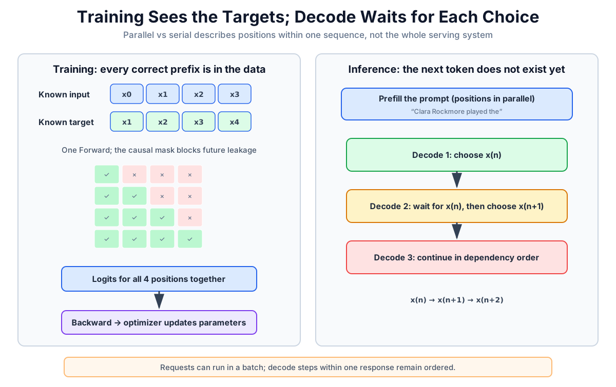
“Parallel” and “serial” refer here to positions within one sequence:
- Training still includes a backward pass; it is not cheaper than one inference call.
- An inference server can batch many requests and run them together.
- Within one answer, however, new token 2 cannot use new token 1 until token 1 has been chosen.
16.1.2 Why Does the Difference Exist?
Use a less forgettable sentence than the usual textbook filler:
- Complete training text: “Clara Rockmore played the theremin without touching it.”
- Inference prompt: “Clara Rockmore played the”
- Training already contains what follows every position; inference does not.
The quoted text is not claiming one visible word equals one token. With GPT-2's tokenizer, for example, “Clara” becomes the two tokens “Cl” and “ara,” while “theremin” in this sentence becomes “ there” and “min.” The model reads token IDs, not the word spacing we see.
16.2 Training in Detail
16.2.1 What Teacher Forcing Means Here
Suppose the tokenizer produces:
Full sequence: [x0, x1, x2, ..., xT]
Model input:   [x0, x1, x2, ..., xT-1]
Targets:       [x1, x2, x3, ..., xT]
The targets are not vaguely “shifted right.” Each target is one token ahead of the input in the same column:
- position 0 reads x0 and predicts x1
- position 1 reads x0, x1 and predicts x2
- ...
- position T-1 reads x0 through xT-1 and predicts xT
Training feeds the ground-truth prefix from the dataset, not the model's sampled guess from the previous position. This is commonly called teacher forcing; for a decoder-only language model, it is the standard next-token training setup.
16.2.2 Why All Positions Can Run Together
Because x0 through xT already exist in the sample, one causally masked matrix computation can produce T positions of logits:
import torch.nn.functional as F

def train_step(model, optimizer, tokens):
    """tokens: [batch, T + 1]; padding omitted for the moment."""
    model.train()
    optimizer.zero_grad(set_to_none=True)

    input_ids = tokens[:, :-1]
    target_ids = tokens[:, 1:]

    logits = model(input_ids)  # [batch, T, vocab_size]
    loss = F.cross_entropy(
        logits.reshape(-1, logits.size(-1)),
        target_ids.reshape(-1),
    )

    loss.backward()   # computes gradients only
    optimizer.step()  # parameters change here
    return loss.detach()
If the batch contains padding, two extra masks are needed: Attention must not read pad keys, and pad targets must not enter the loss. In PyTorch code, those target positions are commonly replaced by -100.
16.2.3 What the Causal Mask Actually Hides
Position t may read x0 through xt, then predicts x(t+1):
position 0 sees: [x0,  -,  -,  -, ...] -> predicts x1
position 1 sees: [x0, x1,  -,  -, ...] -> predicts x2
position 2 sees: [x0, x1, x2,  -, ...] -> predicts x3
The diagonal — the current token — is visible. Tokens after it are hidden. Without the mask, position t could read its answer x(t+1) from a future position and the training objective would leak.
16.3 Inference in Detail
16.3.1 Prefill and Decode
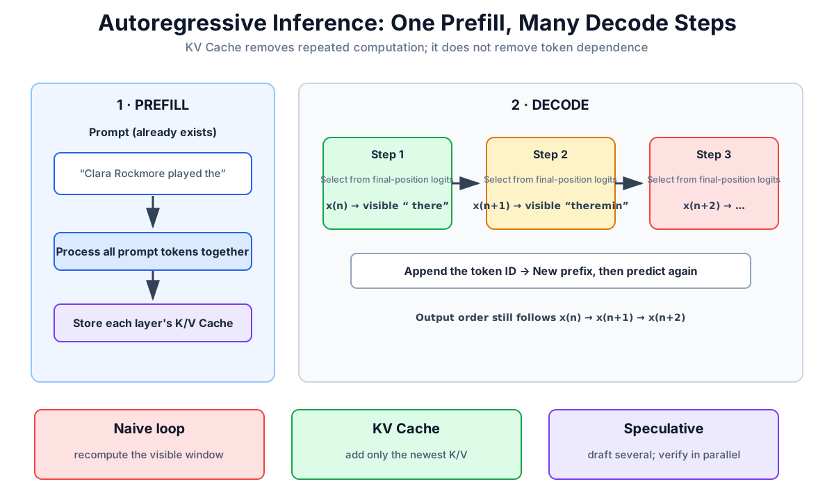
Standard autoregressive inference has two phases:
- Prefill: the complete prompt already exists, so its token positions can be processed together.
- Decode: select a new token from the last-position logits, append it, and only then predict the next one.
Prompt: “Clara Rockmore played the”
          | prefill
Select the next token: “ there”
          | append token ID 612
Select the next token: “min”
          | the visible text now ends in “theremin”
Continue until EOS, a stop condition, or max_new_tokens
That slightly odd “ there” + “min” sequence is the real GPT-2 tokenization of “ theremin.” A decode loop appends token IDs; one token need not be a whole word.
16.3.2 What KV Cache Changes
The simplest code recomputes the whole visible window at every step. KV Cache stores each layer's past Keys and Values:
- prefill computes and stores K and V for the prompt
- decode usually sends only the newest token through the layers and reads the cache
- token choices remain ordered; the cache removes repeated work, not the dependency
Chapter 22 takes that mechanism apart.
2026 update: The standard decode logic is ordered, but speculative decoding can let a smaller model draft several tokens and have the target model verify them in parallel. If the first draft is rejected, the correction step still emits one target-distributed token; when drafts match, an iteration may advance several tokens. This reduces target-model iterations without turning the target model into a non-autoregressive model.
16.3.3 Context Length Is Not an Automatic Sliding Switch
Prompt tokens plus generated tokens must fit the model's supported context. When they do not, the application needs a policy:
- stop generation or reject an overlong input
- truncate older tokens
- summarize older material and put the summary back into context
- use model-native sliding-window Attention
“Always keep the newest N tokens” is one policy, not something every GPT silently does for you. Once a token is removed, it is no longer an input to that forward pass; that is more precise than saying the model psychologically “forgot” it.
16.4 A Baseline Loop Without KV Cache
This deliberately plain version makes the serial dependency visible. It supports batch size 1 and recomputes the current window at every step; it is not a production inference engine.
import torch

@torch.inference_mode()
def generate_greedy(
    model,
    prompt_ids,
    context_length,
    eos_token_id,
    max_new_tokens=50,
):
    """prompt_ids: [1, prompt_length]"""
    if prompt_ids.ndim != 2 or prompt_ids.size(0) != 1:
        raise ValueError("This teaching loop expects batch size 1")

    model.eval()
    generated = prompt_ids.clone()

    for _ in range(max_new_tokens):
        model_input = generated[:, -context_length:]
        logits = model(model_input)
        next_token = logits[:, -1, :].argmax(dim=-1, keepdim=True)
        generated = torch.cat((generated, next_token), dim=1)

        if next_token.item() == eos_token_id:
            break

    return generated
Four details are easy to mix up:
- model.eval() changes the behavior of modules such as Dropout. It does not choose the most likely token.
- torch.inference_mode() disables gradient tracking and more Autograd overhead than no_grad.
- Only the final position's logits are needed to choose the next token.
- argmax makes this greedy decoding. Replace it with sampling and outputs can differ even in eval mode.
16.5 Padding and Batched Inference
16.5.1 Why Left Padding Is Convenient
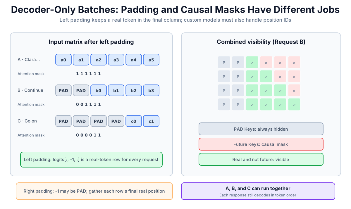
Prompts contain different numbers of tokens, so a batch matrix needs padding. Decoder-only generation often left-pads:
request A: [a0, a1, a2, a3]   mask = [1, 1, 1, 1]
request B: [PAD, PAD, b0, b1] mask = [0, 0, 1, 1]
Now the last column is a real token for every request, so logits[:, -1, :] is convenient. The a and b symbols are tokens; their source text might be “Clara Rockmore played the” and “Continue.”
16.5.2 Do Not Confuse the Two Masks
- Causal mask: do not read future positions.
- Padding mask: do not treat PAD as context.
Implementations usually combine them, converting masked Key scores to negative infinity before Softmax, so their Attention weights become zero. The model does not “learn to ignore padding” during inference; the mask enforces it in that call.
tokenizer.padding_side = "left"
batch = tokenizer(prompts, padding=True, return_tensors="pt")

logits = model(
    batch["input_ids"],
    attention_mask=batch["attention_mask"],
)
next_token_logits = logits[:, -1, :]
With right padding, the last column may be PAD, so blindly taking -1 for every row is wrong; gather each row's last real position instead. A hand-built model with learned absolute positions must also derive correct position IDs for left padding. Mature generation helpers usually do this, but custom code cannot assume it.
Batching and continuous batching let requests share hardware. They improve utilization without removing the token dependency inside each response.
16.6 The Real Compute and Runtime Comparison
| Training | Autoregressive inference | |
|---|---|---|
| Main path per sample | one forward + one backward + optimizer update | one prefill + N dependent decode steps |
| Parallel dimensions | batch, sequence positions, Attention heads | batch and prompt positions; separate requests can run together |
| State to retain | activations, gradients, usually optimizer state | weights and, commonly, KV Cache |
| Common bottlenecks | compute, memory capacity, communication | prefill is compute-heavy; decode is often memory-bandwidth and latency bound |
| Parameters change? | during optimizer.step() | no |
So do not memorize “inference is slower than training.” Training a model costs vastly more total compute than generating one answer. The narrow point is that new tokens in one answer cannot all be computed at once like known training target positions.
16.6.1 Dropout Behavior
If the architecture actually includes Dropout:
model.train()  # Dropout participates in random dropping
model.eval()   # Dropout is disabled
Some modern LLMs configure Dropout as zero. Even when Dropout is disabled, sampling remains random; conversely, low-level numeric nondeterminism can affect greedy runs. eval() means “use evaluation behavior,” not “guarantee identical text.”
16.7 Decoding Strategies
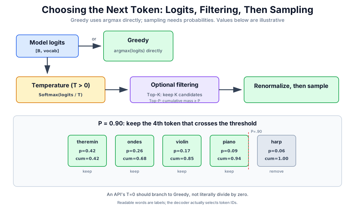
The model produces logits. Choosing the next token is the decoder's job.
16.7.1 Greedy and Direct Sampling
# Greedy needs no Softmax: argmax(logits) == argmax(Softmax(logits))
next_token = logits.argmax(dim=-1, keepdim=True)

# Sampling needs probabilities; temperature must be positive
probs = F.softmax(logits / temperature, dim=-1)
next_token = torch.multinomial(probs, num_samples=1)- Greedy picks the largest logit at every step. It is easy to reproduce, but a local best choice need not make the best sequence and can become repetitive.
- Sampling draws from the distribution. It is more varied and can also select poor low-probability tokens.
- Temperature below 1 sharpens the distribution; above 1 flattens it. An API's “temperature = 0” should branch to greedy rather than literally divide logits by zero.
16.7.2 Correct Top-K Indexing
top_k_probs, top_k_ids = torch.topk(probs, k=50, dim=-1)
sampled_slot = torch.multinomial(top_k_probs, num_samples=1)
next_token = top_k_ids.gather(-1, sampled_slot)
The earlier indexing expression selected the wrong axis when a batch dimension was present. gather converts “which candidate slot?” back into a vocabulary token ID for each row.
16.7.3 Correct Top-P (Nucleus Sampling)
def sample_top_p(logits, top_p=0.9, temperature=1.0):
    if not 0.0 < top_p <= 1.0:
        raise ValueError("top_p must be in (0, 1]")
    if temperature <= 0:
        raise ValueError("temperature must be positive")

    sorted_logits, sorted_ids = torch.sort(
        logits / temperature, descending=True, dim=-1
    )
    sorted_probs = F.softmax(sorted_logits, dim=-1)
    cumulative = torch.cumsum(sorted_probs, dim=-1)

    # Keep the token that first carries cumulative probability to top_p
    remove = cumulative > top_p
    remove[..., 1:] = remove[..., :-1].clone()
    remove[..., 0] = False

    filtered_logits = sorted_logits.masked_fill(remove, float("-inf"))
    filtered_probs = F.softmax(filtered_logits, dim=-1)
    sampled_slot = torch.multinomial(filtered_probs, num_samples=1)
    return sorted_ids.gather(-1, sampled_slot)
The old cumsum <= 0.9 sketch discarded the token that crossed the threshold and could even leave no candidate. Top-P keeps the smallest set whose cumulative probability reaches P, as introduced in the nucleus-sampling paper. Production decoders often combine Temperature, Top-K, and Top-P; they are not mutually exclusive switches.
16.8 Why Are GPT-Style Models Autoregressive?
16.8.1 “Language Has Order” Is Not the Whole Reason
“The luthier repaired the theorbo” and “The theorbo repaired the luthier” plainly differ, but autoregression is not the only way a model can represent order. Autoregressive modeling chooses this probability factorization:
p(x1, x2, ..., xT) = Π p(xt | x1, ..., x(t-1))That gives us:
- a clear next-token objective at every training position
- variable-length generation
- conditioning on both the prompt and generated prefix
- a likelihood that decomposes token by token for training and evaluation
It does not guarantee coherence or factual accuracy. It only lets each step condition on earlier context; quality still depends on the model, data, decoding, and prompt.
16.8.2 Non-Autoregressive Generation Has Not Disappeared
Non-autoregressive translation, iterative masked prediction, and diffusion language models all explore more parallel generation. The 2025 LLaDA paper, for example, reports a large diffusion language model trained from scratch.
So “non-autoregressive is always worse” and “all the best models are autoregressive” are both too absolute. A more durable conclusion is that autoregressive decoders remain a mature and common route, while parallel or iterative generators are real alternatives with different speed and quality tradeoffs.
16.9 Chapter Summary
16.9.1 Core Comparison
| Aspect | Training | Inference |
|---|---|---|
| Targets known? | yes, from the training text | no, selected at runtime |
| Within-sequence work | all target positions together | prefill, then dependent decode steps |
| Compute stages | forward + backward + optimizer | forward only, commonly with KV Cache |
| Dropout | enabled as configured | disabled by eval() |
| Parameter updates | during optimizer.step() | none |
16.9.2 Core Insight
Training is parallel across positions because the correct prefix for each position already exists in the data. Standard inference decode is ordered because one selected token becomes the prefix for the next. KV Cache removes repeated computation, batching parallelizes requests, and speculative decoding reduces target-model iterations; none erases the conditional dependency chain.
Chapter Checklist
After this chapter you should be able to:
- write the one-token offset between inputs and targets using x0 through xT
- explain why the causal mask includes the current token but hides the next one
- distinguish prefill, decode, and KV Cache
- explain why serial single-response decode does not mean all inference is serial
- implement Top-P without dropping the threshold-crossing token
See You in the Next Chapter
The inference path is now clear; Chapter 22 will open up KV Cache in detail. First, there is one sensitive training control left to understand: learning rate. Too large and updates jump past useful regions; too small and progress crawls. Chapter 17 shows what that knob actually controls.