One-sentence summary: no matter how large the model is or how much it cost to train, an LLM can be understood as two things: one file full of parameters and one program that runs inference.

2.1 How Does GPT Answer?

In Chapter 1, we looked at where GPT came from. Now we ask a more basic question:

How does GPT produce an answer one token at a time?

2.1.1 Laying Track in Front of the Train

I like the image of a train laying track just ahead of itself.

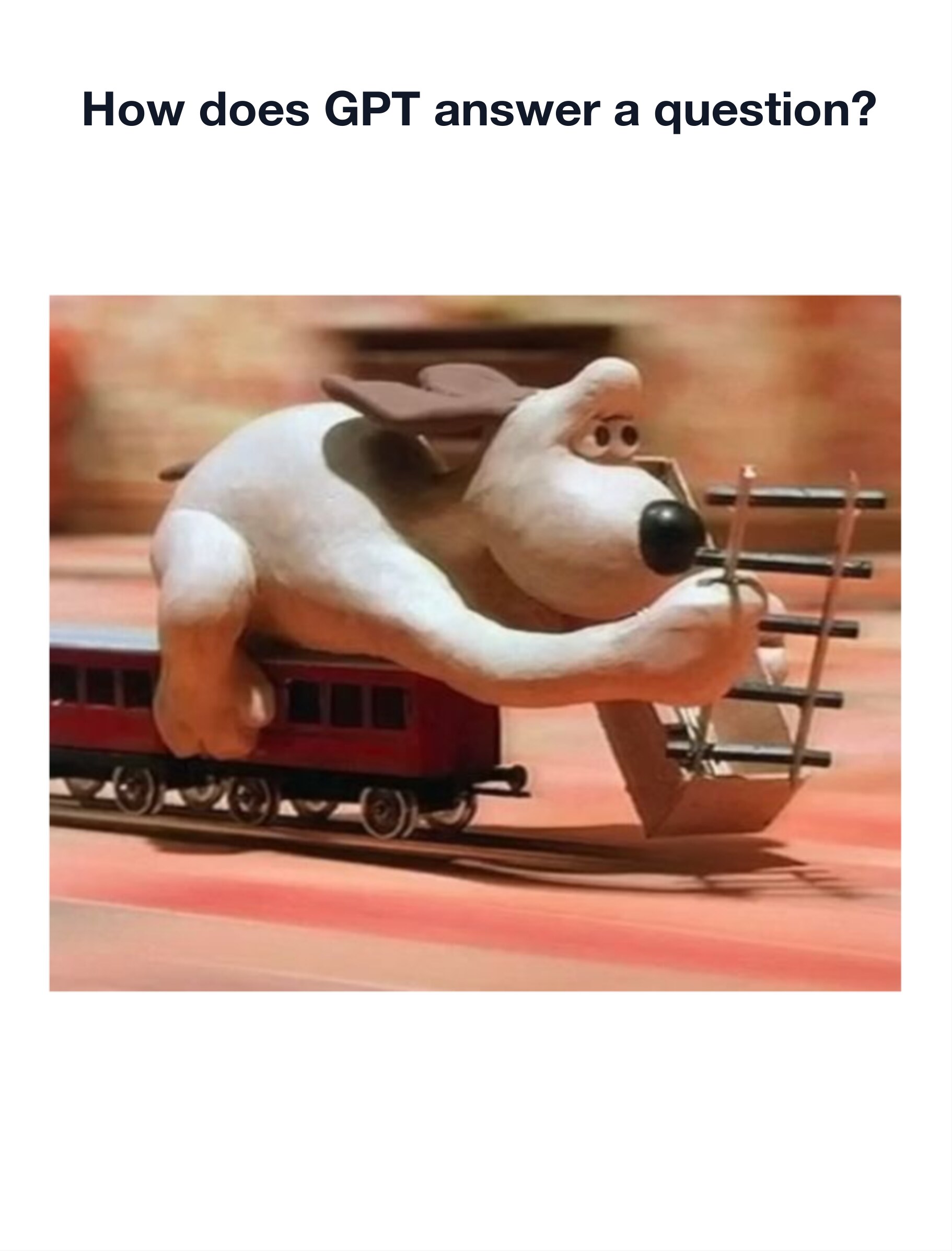
The train cannot jump to the final station. It moves forward by repeating one small action:

1. lay a piece of track
2. move onto that piece
3. lay the next piece
4. move again

GPT generates text in almost the same way:

• train = the model
• track = generated tokens
• laying track = predicting the next token

The model does not usually produce the whole answer in one step. It predicts the next token, appends it to the context, then predicts again.

That is why text appears gradually in a chat interface. It is not theatrical animation. The model is actually generating step by step.

2.1.2 Why Next Token Prediction?

You might ask: why not output the whole answer at once?

Because language has too many possible continuations. A question can have many valid answers, and each answer can be phrased in many ways. Predicting a whole paragraph directly would require choosing from an enormous combinatorial space.

Next token prediction makes the problem manageable:

Given everything so far, what token should come next?

The technical term is autoregressive generation. "Auto" means the model feeds its own previous output back into the next step. The answer grows by using its own prefix as context.

2.2 The Signal Hidden in Text Frequency

If GPT predicts the next token, how does it know what is likely?

2.2.1 A Simple Thought Experiment

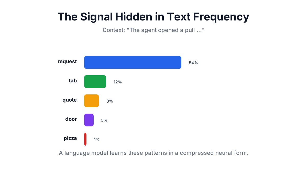
Imagine you see this prefix:

The agent opened a pull ...

What comes next?

Most English speakers expect:

request

That is not magic. It is a statistical pattern. In modern engineering text, "opened a pull request" appears far more often than "opened a pull quote" or "opened a pull tab."

A language model learns patterns like this at massive scale:

• after "opened a pull", "request" is likely
• after "the build turned", "green" is likely
• after "vibe-coded a", "prototype" or "demo" may be likely depending on context

GPT is not a simple frequency table, but frequency is the beginning of the intuition.

2.2.2 From Statistics to Neural Networks

A raw frequency table would be impossible to store. You would need entries for every possible context.

The model solves this by compressing statistical patterns into a neural network.

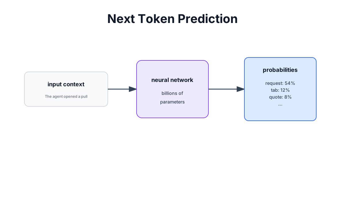
The process looks like this:

• Input: a context such as "The agent opened a pull"
• Neural network: a large set of learned parameters
• Output: a probability distribution over possible next tokens

For example:

The model can then pick the highest-probability token, sample from the distribution, or use a decoding strategy that balances confidence and variety.

Parameters are the model's learned memory. A model with billions of parameters stores billions of numbers that encode patterns learned from text.

2.3 Autoregressive Generation Step By Step

Now let us watch the loop.

2.3.1 Simple Version

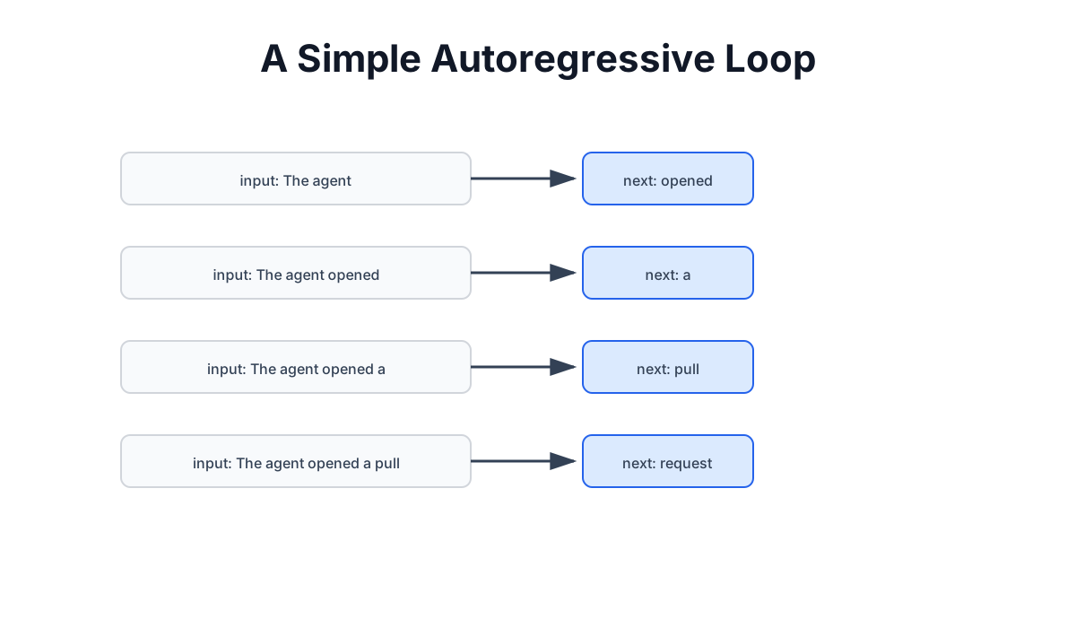
Suppose the prompt begins:

The agent

The model loop might produce:

1. input The agent -> output opened
2. input The agent opened -> output a
3. input The agent opened a -> output pull
4. input The agent opened a pull -> output request
5. input The agent opened a pull request -> output .

At every step, the model uses the full prefix: the user prompt plus all tokens generated so far.

2.3.2 Detailed Version

The repeated pattern is:

context -> model -> next token -> append -> new context

This continues until one of several stopping conditions:

1. the model produces an end-of-text token
2. the system reaches a max token limit
3. the user or application stops generation

2.3.3 Why It Can Feel Slow

Generating 100 new tokens means running the model 100 times. Each step needs the previous context. Later chapters will show how KV Cache avoids recomputing everything from scratch, but the high-level idea remains:

Text generation is a loop, not a single shot.

2.4 What Does Training Require?

Once you understand inference, the next question is training.

To train a large model, you need:

large data + large compute + large engineering effort

2.4.1 Data

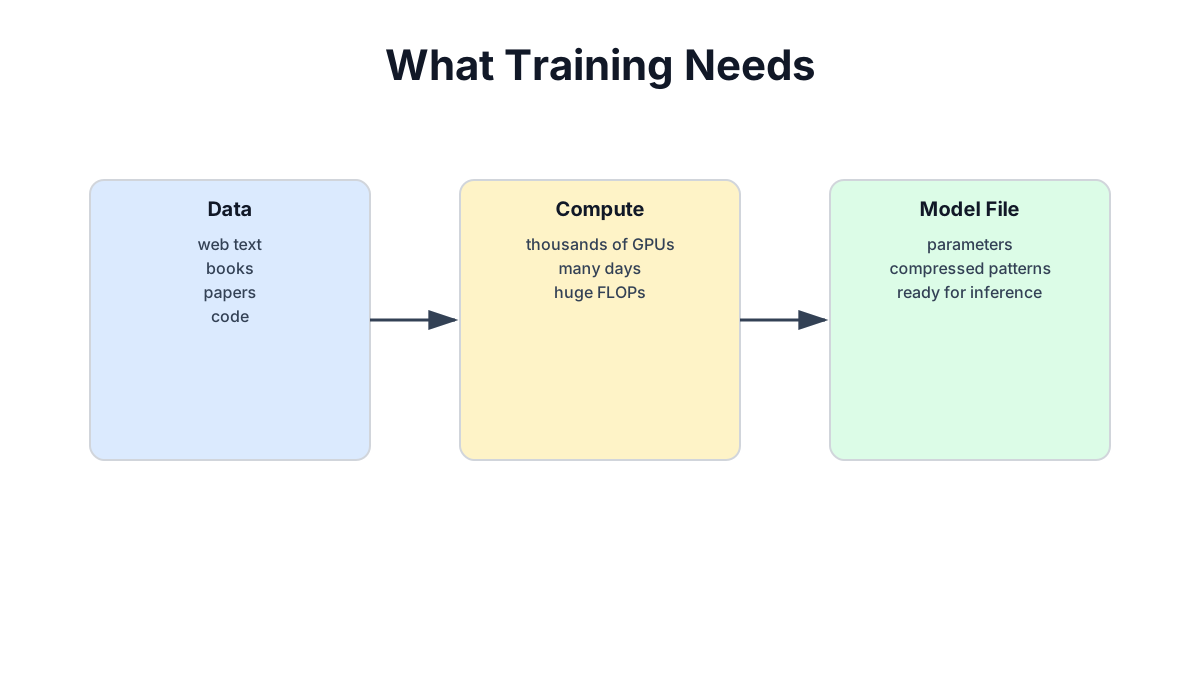
Training data can include:

• web pages
• books
• papers
• code
• instruction data
• human preference data

The data must be cleaned, filtered, deduplicated, and mixed carefully. Bad data does not disappear just because the model is large. Garbage in, garbage out still applies.

2.4.2 Compute

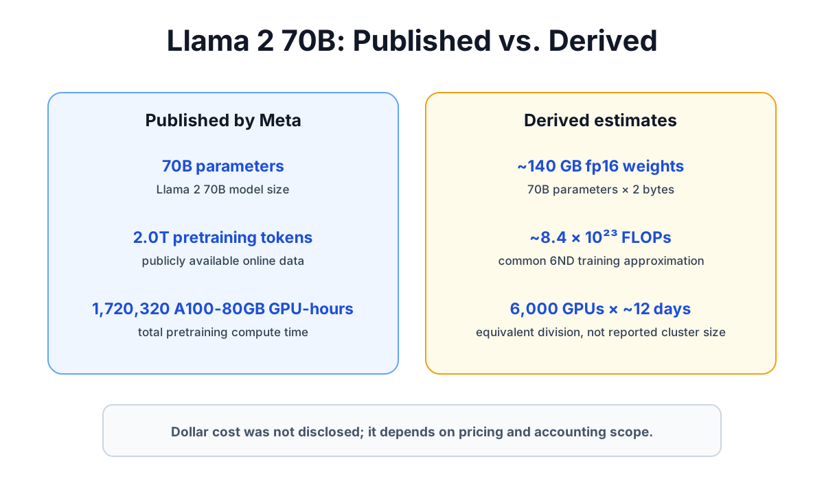
A 70B-class model can require thousands of high-end GPUs running for many days. One useful order-of-magnitude memory hook is: roughly 10 TB of curated text, about 6,000 NVIDIA A100 GPUs, about 12 days of training, and about 10^21 floating point operations.

The exact numbers differ by training recipe, hardware, data mix, and implementation efficiency, so treat those figures as scale intuition rather than a universal invoice. But the direction is stable:

• hardware is expensive
• electricity is expensive
• distributed failures are expensive
• expert engineering time is expensive

This is why people say that frontier models cost millions of dollars to train. A rough public estimate around $2M is a useful anchor for a large run, before remembering that hardware ownership, staffing, failed runs, data work, and serving infrastructure can move the real all-in cost much higher. (Frontier models like GPT-4 are reportedly two orders of magnitude more expensive to train.)

2.4.3 MoE: Bigger Without Activating Everything

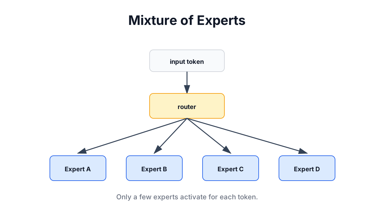
One way to grow model capacity is Mixture of Experts, or MoE.

Instead of activating every parameter for every token, the model uses a router to select a small number of expert networks. This allows the total parameter count to be very large while keeping per-token computation more manageable.

The idea is:

one huge dense model -> many experts, only a few active per token

We will return to MoE in a later chapter.

2.5 The User Sees a Chat Box

After all this machinery, the user sees something simple.

From the user's perspective:

• type a message
• receive an answer
• continue the conversation
• rely on context across turns

Behind that simple interface:

• a neural network maps context to logits
• logits become probabilities
• probabilities become tokens
• tokens become text
• the loop repeats

Understanding this gap between interface and mechanism is the first step to understanding LLMs as engineering systems.

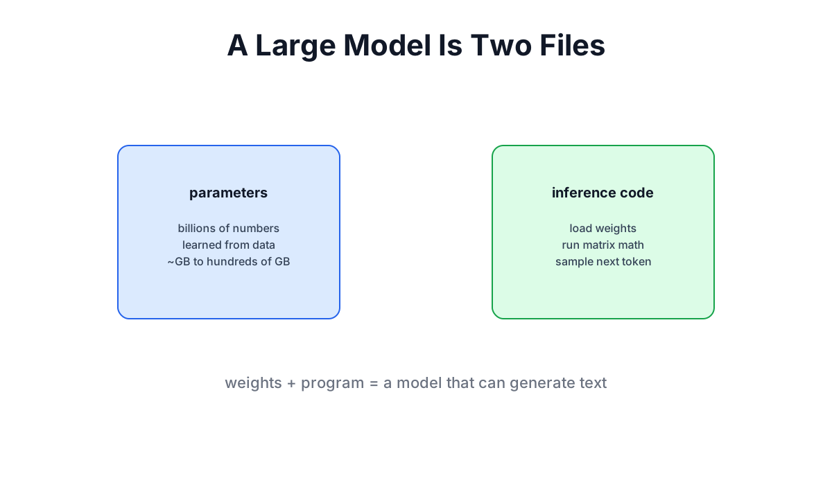
2.6 The Core Idea: A Large Model Is Two Files

Now we arrive at the most important idea in this chapter.

Andrej Karpathy has a useful framing:

A large language model is two files.

What does that mean?

2.6.1 File One: Parameters

The parameter file stores the learned numbers.

For a large model, this file can be many gigabytes. A 70B model stored in fp16 is about 140GB just for the parameters. The numbers inside it are not labels, rules, or hand-written facts. They are floating point values learned during training.

You can think of the parameter file as:

compressed statistical structure learned from data

2.6.2 File Two: Inference Code

The inference code loads the parameters and runs the forward pass:

1. tokenize the input
2. look up embeddings
3. pass through Transformer blocks
4. compute logits
5. sample the next token
6. repeat

Karpathy's llama2.c demonstrated this beautifully: the core inference logic for a LLaMA-style model can be written in about 500 lines of C.

The code is not trivial, but it is not mystical either.

2.6.3 Why This Framing Matters

The "two files" idea helps with several later concepts:

1. Deployment: load parameters, run inference code.
2. Quantization: compress the parameter file.
3. Fine-tuning: adjust some parameters based on new data.
4. LoRA: store small parameter deltas instead of rewriting everything.
5. Serving: make the inference loop fast, batched, cached, and observable.

The magic feeling fades. What remains is math and engineering.

2.7 Chapter Summary

2.7.1 Key Concepts

2.7.2 Numbers to Remember

2.7.3 Core Takeaway

An LLM is not a ghost in the machine. It is a parameter file plus code that repeatedly predicts the next token.

Chapter Checklist

After this chapter, you should be able to:

• Explain autoregressive generation with a simple analogy.
• Describe why next token prediction is a practical training target.
• Explain why generation becomes a repeated loop.
• Explain the "two files" framing.
• Connect parameters, inference code, quantization, and fine-tuning.
• State roughly how many GPUs, dollars, and tokens go into training a 70B model.

See You in the Next Chapter

That is it for this chapter. The important thing is not to memorize every number; it is to stop treating the model as a ghost.

Now that we know the model is parameters plus inference code, we need a map of what the inference code actually does.

Chapter 3 gives that map: the full Transformer flow from input text to output probabilities.