Lesson 18: Trading Cost Modeling and Tradability
Alpha exists = (Gross Alpha - Cost) >0
A Typical Scenario (Illustrative)
Note: The following is a synthetic example to illustrate common phenomena; numbers are illustrative and do not correspond to any specific team/account.
In 2019, a quant team showed me their machine learning strategy:
Backtest Results (2015-2019):
- Annual Return: 45%
- Sharpe Ratio: 2.3
- Maximum Drawdown: 8%
- Monthly Win Rate: 78%
"This is the best strategy we've ever seen!" they said excitedly.
I asked one question: "What's your daily turnover rate?"
Answer: 300%.
This means buying and selling stocks equivalent to 3 times the principal every day.
I asked them to recalculate, adding the following real-world costs:
- Trading commission: 0.03% (round trip)
- Market impact: 0.1% (conservative estimate)
- Slippage: 0.05%
Cost Calculation:
- Daily cost = 300% x (0.03% + 0.1% + 0.05%) = 0.54%
- Annual cost = 0.54% x 252 = 136%

Adjusted Backtest:
- Gross return: 45%
- Cost: -136%
- Net return: -91%
Their "money printer" turned into a "money shredder."
This is why trading cost modeling is so important - it determines whether your Alpha is real or an illusion.
18.1 The True Composition of Costs
18.1.1 Explicit Costs vs. Implicit Costs
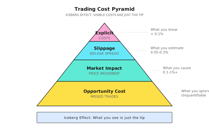
18.1.2 Explicit Costs in Detail
| Cost Type | US Stocks | A-Shares | Cryptocurrency |
|---|---|---|---|
| Commission | 0-0.005% | 0.03% | 0.02-0.1% |
| Stamp Duty | None | 0.1% (sell side) | None |
| Exchange Fees | 0.001% | Included in commission | Included in commission |
| SEC Fees | 0.00008% | None | None |
| Transfer Fees | None | 0.001% | None |
US Stock Explicit Cost Example:
Buying $100,000 of AAPL:
- Commission: $0-5 (depends on broker)
- Exchange fees: ~$1
- Total: ~$5 = 0.005%

Same for selling, round trip about 0.01%
18.1.3 Implicit Costs: The Invisible Killer
Slippage
Definition: The difference between your expected execution price and actual execution price
Expected to buy AAPL at $100.00
Actual execution price $100.05
Slippage = $0.05 = 0.05%
Sources of Slippage:
| Source | Explanation | Influencing Factors |
|---|---|---|
| Bid-Ask Spread | Gap between bid and ask | Liquidity, volatility |
| Price Movement | Time delay from order to execution | Market volatility, network latency |
| Partial Fill | Order split across multiple fills | Order size, order book depth |
Market Impact
Definition: Your trading itself pushes prices in an unfavorable direction
Scenario: You want to buy 10,000 shares of AAPL

Order Book:
  Ask 1: $100.00 x 2,000 shares
  Ask 2: $100.02 x 3,000 shares
  Ask 3: $100.05 x 5,000 shares

If you use a market order to buy all at once:
  First 2,000 shares: $100.00
  Next 3,000 shares: $100.02
  Last 5,000 shares: $100.05

Weighted average price: $100.029
Ideal price: $100.00
Market impact: 0.029%

Moreover: You've consumed Ask 2 and Ask 3
         The next buyer can only buy at higher prices
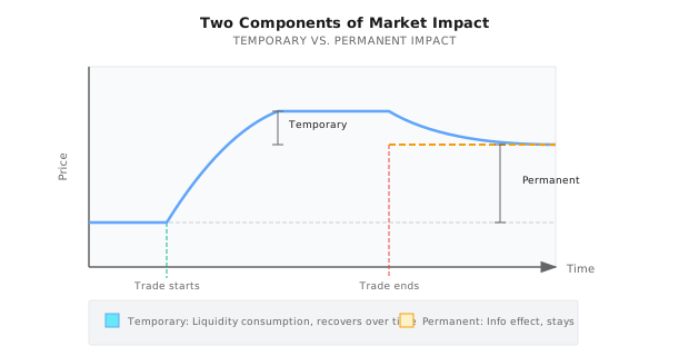
         This is "permanent impact"
Opportunity Cost
Definition: Potential returns lost due to inability to execute or delayed execution
Scenario:
  Price when signal fired: $100
  Your limit order: $99.50
  Price immediately rises to $105
  Your order never fills

Opportunity cost = $105 - $100 = 5%
18.1.4 The Backtest-to-Live Gap Is First a Cost-Accounting Problem
A backtest-to-live gap can come from alpha decay, sampling error, changed exposures, data differences, execution, financing, or accounting. Cost attribution is therefore an early diagnostic, not a universal explanation. Three frequently missed layers are:
Layer one: asynchronous execution accounting. In the IBKR TWS API, execution details and commission reports are separate messages and can be correlated by execId; the API does not promise a fixed arrival delay. Treat fills and fees as events that may arrive separately, make updates idempotent, allow accounting records to remain provisionally incomplete, and finalize them through execution and statement reconciliation. Monitoring execDetails as well as orderStatus is important because not every execution necessarily produces a new order-status message.
Layer two: currency normalization. A multi-currency portfolio must define trade currency, settlement currency, base currency, FX timestamp, and conversion source. P&L, exposure, cash, fees, financing, and backtests must use the same policy; otherwise apparently small unit errors can become large risk errors.
Layer three: fee schedules. Broker, exchange, clearing, regulatory, borrow, financing, and tax charges vary by account, venue, instrument, side, and date. Store versioned fee rules and reconcile modeled costs with statements rather than embedding one broker's current tariff in strategy code.
Do not use universal basis-point cutoffs. Define materiality before launch from the strategy's expected edge, turnover, sample uncertainty, and risk budget. Attribute the gap into signal, market regime, execution, fees, financing, FX, and data revisions; attach confidence intervals and escalate whichever component exceeds its pre-registered tolerance.
18.2 Slippage Modeling
18.2.1 Linear Model
The simplest model assumes slippage is proportional to order size:
Slippage = k x OrderSize / ADV

Where:
- k = empirical coefficient (typically 0.1-0.5)
- OrderSize = order amount
- ADV = Average Daily Volume
Paper Exercise:
You want to buy $500,000 of stock, assuming k = 0.3
| Stock | ADV | Order Ratio | Expected Slippage |
|---|---|---|---|
| AAPL | $10B | 0.005% | 0.3 x 0.005% = 0.0015% |
| TSLA | $3B | 0.017% | 0.3 x 0.017% = 0.005% |
| Small Cap X | $10M | 5% | 0.3 x 5% = 1.5% |
Discovery: On small caps, a $500K order could generate $7,500 in slippage!
18.2.2 Square-Root Model
A more precise model considers nonlinear relationships:
Slippage = k x sigma x sqrt(OrderSize / ADV)

Where:
- sigma = daily volatility
- k = empirical coefficient (typically 0.5-1.5)
Paper Exercise:
| Stock | Volatility sigma | ADV | Order | Slippage (k=1) |
|---|---|---|---|---|
| AAPL | 1.5% | $10B | $1M | 1.5% x sqrt(1M/10B) = 0.015% |
| AAPL | 1.5% | $10B | $100M | 1.5% x sqrt(100M/10B) = 0.15% |
| Small Cap | 3% | $10M | $1M | 3% x sqrt(1M/10M) = 0.95% |
Key Findings:
- Slippage grows sub-linearly with order size (square root relationship)
- High volatility stocks have larger slippage
- Small cap slippage can be 60x that of large caps
18.2.3 Estimating Slippage with Tick Data
With Level-2 data, you can estimate more precisely:
Method: Simulate order walking through the order book

1. Obtain historical order book snapshots
2. Simulate market order consuming each level
3. Calculate weighted average price vs. mid-price
4. Gather slippage distribution for different order sizes
Code Framework (Engineer Reference)
def estimate_slippage(order_size: float,
                     order_book: dict,
                     side: str = 'buy') -> float:
    """
    Estimate slippage based on order book data

    order_book = {
        'bids': [(price1, size1), (price2, size2), ...],
        'asks': [(price1, size1), (price2, size2), ...]
    }
    """
    if side == 'buy':
        levels = order_book['asks']  # Buying consumes asks
    else:
        levels = order_book['bids']  # Selling consumes bids

    mid_price = (order_book['bids'][0][0] + order_book['asks'][0][0]) / 2
    filled = 0
    cost = 0

    for price, size in levels:
        if filled >= order_size:
            break
        fill_amount = min(size, order_size - filled)
        cost += fill_amount * price
        filled += fill_amount

    if filled < order_size:
        # Order book depth insufficient for full execution
        return float('inf')

    avg_price = cost / order_size
    slippage = (avg_price - mid_price) / mid_price

    return slippage if side == 'buy' else -slippage
18.3 Market Impact Modeling
18.3.1 Temporary Impact vs. Permanent Impact
18.3.2 Almgren-Chriss Model
This is the most famous market impact model:
Total Cost = Temporary Impact + Permanent Impact + Volatility Risk

Where:
  Temporary impact is proportional to trading speed (volume per unit time)
  Permanent impact is proportional to total trading volume
  Volatility risk is proportional to execution time x volatility

Trade-off:
  Trade fast -> High temporary impact, but low volatility risk
  Trade slow -> Low temporary impact, but high volatility risk
Intuitive Explanation:
Imagine pouring a bucket of water into a pond. Pour fast (all at once) -> Big splash (temporary impact), but water settles quickly Pour slow (drop by drop) -> Small splash, but wind and rain may occur during (volatility risk)
18.3.3 Paper Exercise: Execution Strategy Selection
You want to buy $10M of AAPL (ADV = $10B), volatility = 1.5%/day
| Execution Strategy | Execution Time | Temporary Impact | Volatility Risk | Total Cost |
|---|---|---|---|---|
| Single market order | Instant | High | None | High |
| 10 orders (1 day) | 1 day | Low | 1.5% | Medium |
| 50 orders (5 days) | 5 days | Very low | 3.4% | Potentially higher |
Optimal Solution: Balance based on urgency and risk preference
18.4 Tradability Assessment
18.4.1 Fill Probability Modeling
The Limit Order Problem: Your orders may not get filled
Fill probability P(fill) depends on:
1. Distance of limit price from current price
2. Queue depth at the price level
3. Price volatility range
4. Waiting time

Estimation formula (simplified):
P(fill) ~ 1 - exp(-lambda x time)

Where lambda relates to price distance and volatility
Paper Exercise:
You place a $99 limit buy order on a $100 stock (1% below market)
| Scenario | Daily Volatility | Expected Fill Probability |
|---|---|---|
| Low volatility | 0.5% | ~20% (hard to reach -1%) |
| Medium volatility | 1.5% | ~60% (often reaches) |
| High volatility | 3% | ~85% (almost certainly reaches) |
Problem: High fill probability means prices often drop - might not be a good signal
18.4.2 Liquidity Cost Metrics
| Metric | Formula | Meaning |
|---|---|---|
| Order Ratio | Order / ADV | Lower is better |
| Liquidity Consumption | Order / Order Book Depth | Lower is better |
| Waiting Cost | Signal Decay x Wait Time | Lower is better |
| Total Cost | Slippage + Impact + Opportunity Cost | Total cost |
18.4.3 Alpha Purification: From Gross to Net
Gross Alpha: Predicted return (from backtest)

Minus:
  - Explicit costs (commission, taxes)
  - Slippage (Bid-Ask + latency)
  - Market impact
  - Opportunity cost

Equals:
  Net Alpha: Actually achievable return

Key Formula:
  Strategy viable <=> Net Alpha >0
  Strategy viable <=> Gross Alpha > Total Cost
Paper Exercise:
| Strategy | Gross Alpha | Turnover | Cost Per Trade | Annual Cost | Net Alpha |
|---|---|---|---|---|---|
| A | 15% | 50% | 0.2% | 2% | 13% |
| B | 20% | 200% | 0.2% | 8% | 12% |
| C | 30% | 500% | 0.2% | 20% | 10% |
| D | 40% | 1000% | 0.2% | 40% | 0% |
| E | 50% | 2000% | 0.2% | 80% | -30% |
Findings:
- Strategy E has highest gross Alpha but lowest net return
- Strategy A has lowest gross Alpha but highest net return
- High turnover is the Alpha killer
18.5 Strategy Crowding: When Everyone Trades the Same Signal
Cost modeling focuses on your own orders. But there is a systemic cost that no individual model can estimate: what happens when hundreds of funds hold the same positions and try to exit at the same time.
Case Study: 2024 China Small-Cap Quant Crisis
In early 2024, many of China's top quantitative funds suffered simultaneous drawdowns of 8-13% within weeks. Ubiquant, Lingjun, and High-Flyer -- firms managing tens of billions -- all posted double-digit losses in their CSI 500 enhanced products. The cause was not a single bad trade but strategy homogenization: most funds had overweighted small and micro-cap stocks using similar momentum and size factors. When regulatory tightening restricted micro-cap trading, forced liquidations triggered a positive feedback loop -- selling compressed liquidity, which forced more selling. Backtested slippage models, calibrated on normal conditions, wildly underestimated the impact.
The lesson: your cost model must account for crowding risk. If your strategy uses widely published factors on capacity-constrained stocks, your true cost includes the tail risk of correlated unwinding.
For a deeper analysis of strategy homogenization dynamics, capacity estimation methods, and countermeasures, see Background: Strategy Homogenization and Capacity Bottlenecks.
18.6 Why Many ML Alphas Are Untradable
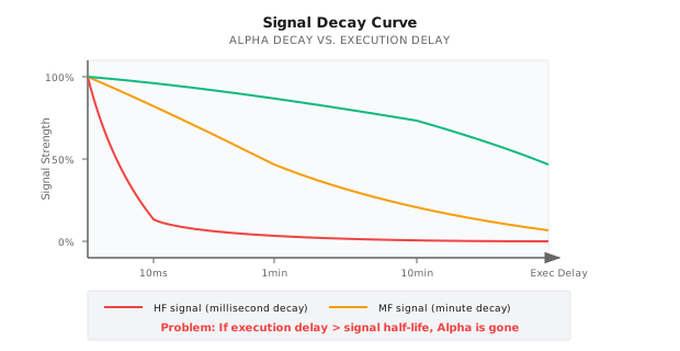
18.6.1 Signal Decay Rate vs. Execution Delay
18.6.2 Capacity Constraints of High-Frequency Alpha
| Alpha Type | Typical Decay | Capacity | Viability |
|---|---|---|---|
| Market Making | Milliseconds | $1-10M | Requires HFT infrastructure |
| Statistical Arbitrage | Seconds-minutes | $10-100M | Requires low latency |
| Technical Momentum | Minutes-hours | $100M-1B | Retail possibly viable |
| Fundamental Factors | Days-weeks | $1B+ | Ample capacity |
Key Insight:
ML models easily discover short-term Alpha (because signal-to-noise ratio is high) But these Alphas often decay too fast for retail traders to execute
18.6.3 Case Study: High Win-Rate Strategy's Live Trading Collapse
Backtest Results:
- Daily win rate 65%
- Daily average return 0.3%
- Sharpe 3.0
Strategy Characteristics:
- Signal decay half-life: 2 minutes
- Average execution delay: 5 minutes
Problem:
When signal fires: Expected return +0.5%
After 2 minutes: Expected return +0.25% (50% decay)
After 5 minutes (actual execution): Expected return +0.06%

Minus 0.1% cost: Net return -0.04%

65% win rate x (-0.04%) = Continuous losses
18.7 Multi-Agent Perspective
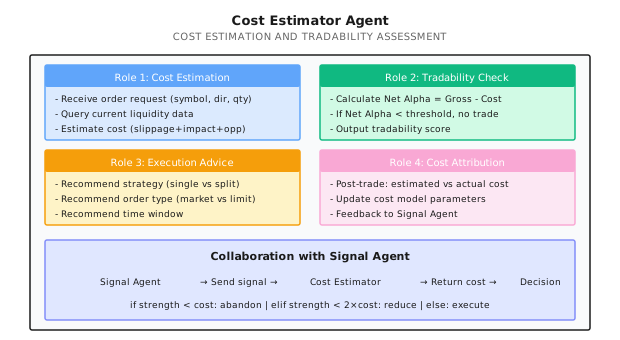
18.7.1 Cost Estimator Agent
18.7.2 Cost-Aware Strategy Design
| Design Principle | Implementation |
|---|---|
| Reduce turnover | Extend holding period, raise signal threshold |
| Select high liquidity assets | Filter stocks with ADV < threshold |
| Avoid high volatility periods | No trading at open/close/events |
| Use smart orders | TWAP, VWAP, algorithmic trading |
| Capacity management | Strategy capacity = f(liquidity, impact) |
Acceptance Criteria
After completing this lesson, use the following criteria to verify learning:
| Criterion | Standard | Self-Test Method |
|---|---|---|
| Understand cost composition | Can list explicit and implicit costs | Draw cost pyramid |
| Estimate slippage | Can calculate slippage using square-root model | Complete paper exercises |
| Understand market impact | Can explain temporary and permanent impact | Give examples |
| Assess tradability | Can calculate Net Alpha | Evaluate a strategy |
| Understand ML Alpha traps | Can explain signal decay problem | Analyze a high-frequency strategy |
Lesson Deliverables
After completing this lesson, you will have:
- Cost Classification Framework - Explicit, implicit, opportunity costs
- Slippage Estimation Models - Linear and square-root models
- Tradability Assessment Method - Gross Alpha to Net Alpha
- Cost Estimator Agent Design - Cost estimation and decision collaboration
Key Takeaways
- Trading cost = Explicit cost + Slippage + Market impact + Opportunity cost
- Slippage has a square-root relationship with order size/ADV
- Strategy viability = Net Alpha >0 = Gross Alpha > Total Cost
- High turnover is the Alpha killer
- ML Alpha easily discovers short-term signals, but execution delay may make them uncapturable
Further Reading
- Lesson 19: Execution System - From Signal to Real Fill - More details on execution
- Background: HFT and Market Microstructure - Market microstructure basics, Kyle's Lambda
- Background: Execution Simulator Implementation - Code implementation of 4-level execution simulator
- Appendix A: Live Trading Logging Standards - What data to record
Next Lesson Preview
Lesson 19: Execution System - From Signal to Real Fill
Cost modeling tells us "how expensive trading is." In the next lesson, we dive into execution: How to design orders? How to handle slippage? How to turn signals into actual fills in real markets?