DiffusionBlocks: The Network Already Knew It Was Three Parts

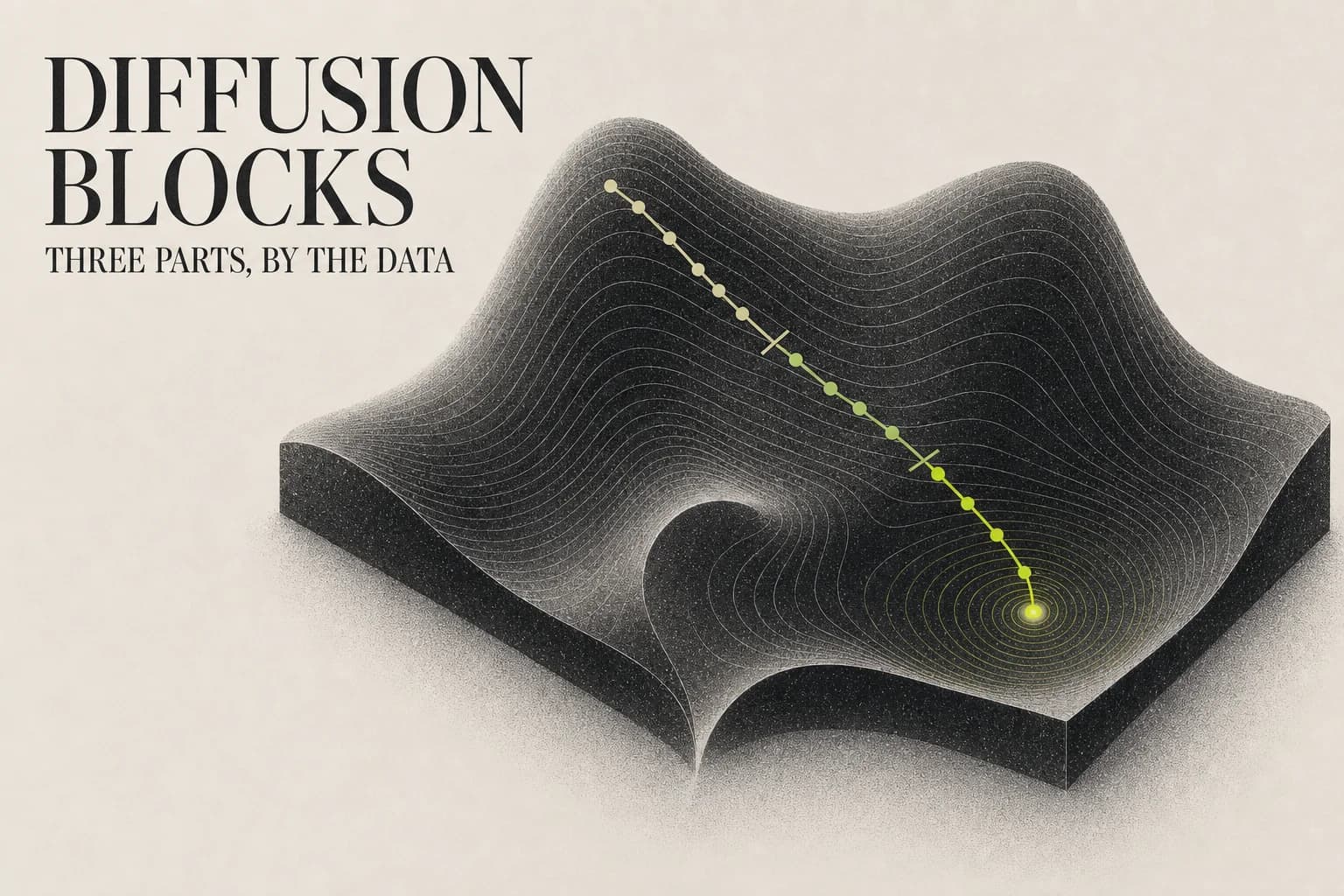
The most expensive line in modern AI training is not the matrix multiply. It is the activation buffer.

End-to-end backpropagation requires holding the activations of every layer alive until the backward pass arrives. For a 24-layer transformer, that means 24 snapshots of the residual stream sitting in GPU memory at once. Scale depth, and you scale the memory bill in lockstep. This is why the 100B-parameter training runs need hundreds of A100s, and why most researchers have never trained anything remotely that large.

Sakana AI's DiffusionBlocks (ICLR 2026) dissolves this constraint. The framework is validated across five architecture families — ViT, DiT, autoregressive, recurrent-depth, and masked diffusion — and the headline result is blunt: block-wise training matches end-to-end performance while cutting peak training memory by roughly the block count. Their paper is clear and worth reading on its own terms. But the question it does not fully answer surfaces in the block-count ablation: why does a small B — and B=3 in particular — work so consistently?

I think the answer is already in the residual stream data, and it connects directly to the manifold view of what neural networks are doing.

What DiffusionBlocks Actually Does

The paper's core insight is that residual connections are not just a skip-gradient trick. They are Euler discretization steps of the probability flow ODE:

Each residual block update z_l = z_{l-1} + f(z_{l-1}) is one Euler step along this trajectory — one denoising step in the reverse diffusion process. The network, already structured this way, can be partitioned into B blocks, each assigned a contiguous noise level range [σ_high, σ_low]. Each block then learns the score function (the denoising direction) for its assigned range via score matching loss, completely independently of the other blocks.

For a 12-layer ViT with B=3, the paper's experimental setup (Section 5.1) is exactly this: three blocks of four layers each, each trained on its own σ range, assembled in sequence at inference. Memory drops to 4 active layers at any training moment instead of 12.

Crucially: no learned connector module is inserted between blocks. The block decomposition governs how the training signal is computed, not the model's architecture. A discriminatively-trained model (the ViT classifier) runs the same forward pass it always did; a generative model runs the usual diffusion sampling loop — one ODE-solver step per noise level, each routed to the block that owns that σ range. Either way, the blocks are stitched together by machinery that already existed, not by anything the method bolts on.

The Block Count Problem

The paper's ablation on DiT shows something worth pausing on:

B=2 and B=3 both beat the end-to-end baseline on FID. B=4 and B=6 start degrading. The paper explains this through diffusion theory: equi-probability partitioning of the noise range works best when each block gets a learning task that is balanced in difficulty. Too few blocks and you waste the independence property. Too many blocks and each block's assigned σ range is too narrow to learn anything globally coherent.

That's the theoretical explanation. But there is a structural one underneath it.

The Empirical Case: The Network Was Already Trifurcated

Earlier this year I ran a layer sweep on a 32-layer Llama 3.1 transformer, measuring the residual stream's correlation (r) at representative layers (notebook here):

Layer  1: r = 0.5091
Layer  4: r = 0.3478  ← minimum: maximum active reshaping
Layer  8: r = 0.3827
Layer 12: r = 0.4139
Layer 16: r = 0.6489  ← step change: manifold consolidating
Layer 20: r = 0.6782
Layer 24: r = 0.7279
Layer 28: r = 0.8540  ← plateau: stable task representations
Layer 30: r = 0.8112
Layer 32: r = 0.8250

Read this in the 指玄境 frame — the Pointing-Mystery Realm, where training is the geometric flattening of a manifold. The r here measures behavioral isometry: at a given layer, how faithfully the geometry of concepts in the residual stream mirrors the geometry of the model's output behavior. Low r means the activation geometry does not yet track behavior — the manifold is still being actively deformed into shape. High r means the two are aligned — the manifold has been found, and subsequent layers refine on a fixed geometric base.

Three phases are visible without squinting:

Phase 1 (layers 1–~10): Embedding flattening. Low, dipping r. The token embeddings arrive tangled — France, 法国, and the concept of a European nation all need to end up pointing at the same geometric region. These layers are actively rotating, stretching, and cutting the ambient space, doing the topological work of manifold separation. The r dips to 0.34 at layer 4 — the point of lowest behavioral isometry, where the activation geometry least resembles the output structure it will eventually encode.

Phase 2 (layers ~10–22): Geometric manifold construction. The rising r from ~0.41 to ~0.67. The manifolds have been roughly separated; now they need to be shaped into the smooth, linearly-separable surfaces that make downstream classification or generation tractable. This is where the network develops what Olah's manifold topology work calls the "clean geometric structure" — the curved surfaces become progressively flatter, and the Muon-optimal geometry begins to solidify.

Phase 3 (layers ~22–32): Task following and generalization. r stabilizes above 0.75 and climbs to 0.85. The manifold is essentially found. These layers are not restructuring geometry — they are applying task-specific transformations to a stable geometric substrate. The residual stream is drifting toward final answer space rather than reorganizing.

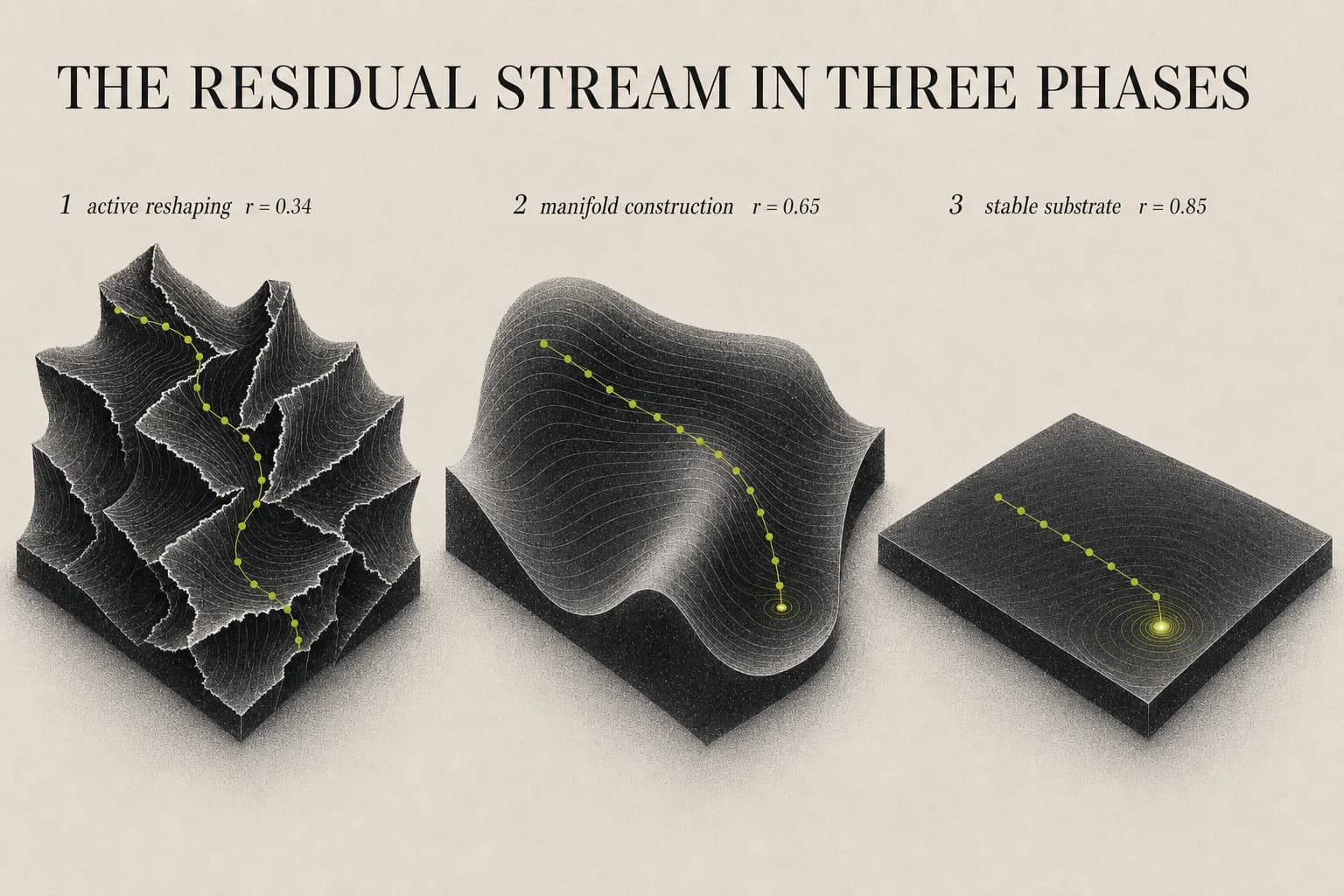
This is not a post-hoc interpretation — it is what the correlation structure of the residual stream looks like before you know about DiffusionBlocks. The network has independently discovered a natural trifurcation.

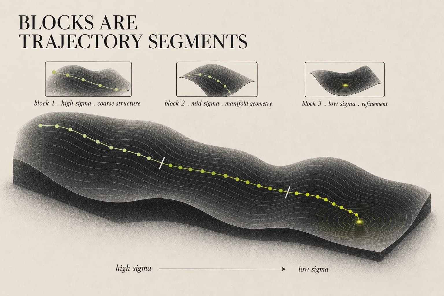
One caveat: the sweep above is a 32-layer decoder LLM, while DiffusionBlocks is validated on ViT, DiT, and others — so I'm treating the three-phase structure as a general property of deep residual stacks rather than something proven architecture-by-architecture. With that said: when DiffusionBlocks assigns B=3 blocks to a 12-layer model, it is partitioning a structure that already exists functionally. Block 1 handles the high-σ range where coarse structure forms — this is the embedding-flattening phase. Block 2 handles mid-σ — manifold geometry. Block 3 handles low-σ — task refinement. The equi-probability partition the paper proposes — equal probability mass per block, which need not land on equal layer boundaries — falls, not by design, near the natural phase structure of the residual stream.

This is why quality holds through B=3 and then erodes: B=4 slips behind B=2/B=3 (though it still edges the end-to-end baseline), and by B=6 it drops below baseline entirely. The network has three structural phases; cutting at two or three boundaries lands at or inside the natural seams, while cutting finer divides a single phase across blocks that each see too little of it to learn a coherent denoising task. The functional structure resists being cut finer than it is.

It also explains the number a naive "three is the magic number" reading would trip on: B=2 (9.90) actually edges out B=3 (11.11) on FID. The phases aren't hard walls — they're soft regimes. The Phase-2→Phase-3 transition in the r-curve is a smooth ramp (0.41 → 0.67 → 0.85), so a three-way cut has to place one boundary inside that ramp, while a two-way cut — active reshaping vs. everything after — splits difficulty more cleanly. So the trifurcation sets the ceiling on useful blocks, not a single optimum. B=3 is the sweet spot for training specifically: it buys 3× memory at near-best quality, and the structural ceiling is what makes paying so little for it safe.

The ODE Connection

The Diamond Realm (金刚境) of the 四境 (Four Realms) framework already made this claim: forward propagation is Euler integration of an ODE. DiffusionBlocks formalizes exactly this at the training level. The residual connection is not just "ODE-like" in a loose sense — it is a specific Euler discretization of the probability flow ODE from score-based diffusion theory, equation (1) in the paper. The dynamical system perspective was always implicit; DiffusionBlocks makes it load-bearing.

The practical consequence: you can now train the ODE one trajectory segment at a time. Blocks are trajectory segments. The three segments correspond to the three geometric phases. This is what makes the independence property work — each segment of the ODE trajectory has its own local score function, which can be learned without global information about the rest of the trajectory.

What This Changes (and What It Doesn't)

What it changes: memory scaling during training. This is genuine and important. A well-tuned B=3 partition means you only need the memory budget for 1/3 of the network at any time. For practitioners training large models on constrained hardware, this is not a minor win.

What it doesn't change: the fundamental geometry of what the network is learning. What the paper actually demonstrates is performance parity — a DiffusionBlocks-trained ViT matches the end-to-end model, and at B=2–3 beats it on FID. It does not measure the learned geometry directly. But the manifold view tells you why parity should hold: the training path is different; the destination is the same fixed point on the manifold space. Same geometry, reached two ways — that is my reading, and the parity numbers are exactly the footprint it would leave.

This is what the manifold view predicts: if many valid paths lead to the same well-flattened manifold geometry, then any principled local objective that navigates each path segment correctly will converge there. DiffusionBlocks gives each block a principled local objective (score matching on its σ range) rather than an ad-hoc auxiliary loss — which is why it works where earlier block-wise methods (Forward-Forward, greedy layer-wise training) struggled.

The Broader Pattern

DiffusionBlocks joins a growing list of papers that are, from the manifold view, rediscovering the same structural truth through different experimental lenses:

• DeepSeek V4's loss spike defenses (manifold tearing post) — three independent engineering solutions to what is geometrically the same problem: sudden deformation of the residual stream manifold
• Muon optimizer — orthogonal weight updates preserve the geometric structure the manifold view says matters; empirically wins on NanoGPT speedruns
• DiffusionBlocks — local training objectives aligned to the ODE trajectory's natural phase structure work because the functional decomposition is real, not imposed

The pattern is: every time someone finds a principled local objective that respects the natural phase structure of the residual stream, it works as well as global backpropagation and often better. The network has always wanted to be three parts. It is taking us a while to notice.

The DiffusionBlocks paper: arxiv.org/abs/2506.14202
Layer sweep notebook: github.com/waylandzhang/manifold-steering-demo-n-critique
Four Realms framework: waylandz.com/blog/four-realms-of-neural-networks

中文版 · DiffusionBlocks：网络一直知道自己是三段式的

现代 AI 训练中最贵的一行代码不是矩阵乘法，而是激活缓冲区。

端到端反向传播要求把每一层的激活值保留到反向传播经过为止。24 层 Transformer 意味着同时在显存里保留 24 份残差流快照。加深网络，显存开销线性增长。这就是为什么百亿参数训练跑需要几百张 A100，也是为什么大多数研究者从未训练过规模接近的模型。

Sakana AI 的 DiffusionBlocks（ICLR 2026）消解了这个约束。这套框架在五类架构上得到验证——ViT、DiT、自回归、recurrent-depth、masked diffusion——结论很直白：块级训练能与端到端性能持平，同时把训练峰值显存压低到大约原来的「1/块数」。 论文值得直接读。但它没有完整回答的问题出现在块数消融里：为什么小的 B——尤其是 B=3——如此一致地好用？

我认为答案已经藏在残差流数据里，而且它直接连接到神经网络的流形观。

DiffusionBlocks 究竟做了什么

论文的核心洞察是：残差连接不只是跳梯度的技巧，它们是概率流 ODE 的欧拉离散化步骤：

每个残差 block 的更新 z_l = z_{l-1} + f(z_{l-1}) 是沿这条轨迹走一步欧拉步——反向扩散过程中的一次去噪步骤。网络已经是这个结构，因此可以被切成 B 块，每块分到一段连续的噪声级别区间 [σ_high, σ_low]，各自用 score matching 损失独立训练该区间的去噪方向，彼此完全不需要梯度通信。

12 层 ViT 用 B=3 就是这样：三块各四层，各自训练，推理时顺序拼接。任一训练时刻只需要 4 层的激活，而不是 12 层。

重点：block 之间没有插入任何需要学习的连接模块。 块的划分管的是训练信号怎么算，而不是模型的架构。判别式训练的模型（ViT 分类器）推理时跑的还是原来那条前向通路；生成式模型推理时跑的是常规的扩散采样循环——每个噪声级别走一步 ODE 求解，交由拥有该 σ 区间的块负责。两种情况下，把块串起来的都是本就存在的机制，而不是这套方法新加的东西。

Block 数量的问题

论文在 DiT 上的消融实验值得停下来看一眼：

B=2 和 B=3 都超过了端到端基线的 FID。B=4 和 B=6 开始退化。论文用扩散理论解释：对噪声区间做等概率划分时，每块的学习难度最均衡。块数太少浪费独立性；块数太多，每块分到的 σ 区间太窄，学不到全局连贯的东西。

这是理论解释。但底层还有一个结构性解释。

实证依据：网络本来就是三段式的

今年早些时候我在 32 层 Llama 3.1 上跑了一个层扫描实验，测量残差流在各层的相关系数 r（notebook）：

Layer  1: r = 0.5091
Layer  4: r = 0.3478  ← 最低点：几何变形最剧烈
Layer  8: r = 0.3827
Layer 12: r = 0.4139
Layer 16: r = 0.6489  ← 阶跃：流形开始固化
Layer 20: r = 0.6782
Layer 24: r = 0.7279
Layer 28: r = 0.8540  ← 高原：任务表示趋于稳定
Layer 30: r = 0.8112
Layer 32: r = 0.8250

用指玄境的框架来读。这里的 r 衡量的是行为同构性（behavioral isometry）：在某一层上，残差流里概念的几何结构在多大程度上忠实地映照模型输出行为的几何结构。低 r 说明激活几何还没对齐行为——流形仍在被主动形变成形。高 r 说明两者已经对齐——流形已经被找到，后续层在已固定的几何基底上精调。

三个阶段一眼可见：

第一阶段（第 1–约 10 层）：Embedding 展平。 r 低且下探。词元 embedding 进来是缠绕的——法国、France、欧洲大陆国家这几个概念需要最终指向同一个几何区域。这些层在主动旋转、拉伸、切割环境空间，做的是流形分离的拓扑工作。第 4 层 r 跌到 0.34——行为同构性最低的一点，此处激活几何与它最终要编码的输出结构最不相像。

第二阶段（约第 10–22 层）：几何流形构建。 r 从约 0.41 缓缓升到约 0.67。流形粗略分离了；现在需要把它们塑造成平滑、线性可分的曲面。这里网络发展出 Olah 流形拓扑工作 所说的"干净几何结构"，弯曲的曲面逐渐展平，Muon 意义上的最优几何开始固化。

第三阶段（约第 22–32 层）：任务跟随与泛化。 r 稳定在 0.75 以上，爬升到 0.85。流形基本被找到。这些层不在重构几何——它们在稳定的几何基底上施加任务相关变换，残差流在漂向最终答案空间，而不是在重组。

这不是事后解读——这是在不知道 DiffusionBlocks 之前，残差流相关结构本来的样子。网络已经自发地找到了三段式划分。

一句限定：上面的扫描是一个 32 层解码器 LLM，而 DiffusionBlocks 验证的是 ViT、DiT 等架构——所以我把这种三段式当作深层残差栈的一般性质，而非逐一架构证明过的结论。在此前提下：DiffusionBlocks 把 12 层模型分成 B=3 块时，切割的正是这个已经功能性存在的结构。第一块处理高 σ 区间（粗粒度结构形成——对应 embedding 展平阶段），第二块处理中 σ（流形几何），第三块处理低 σ（任务精调）。论文提出的等概率划分——每块分到相等的概率质量，未必落在相等的层边界上——并非设计使然地落在了残差流自然相态结构的附近。

这也解释了为什么质量能撑到 B=3、之后开始滑落：B=4 落后于 B=2/B=3（但仍略胜端到端基线），到 B=6 就彻底跌破基线。网络有三个结构阶段，切两到三刀正好落在自然接缝处或附近，再往细切就会把同一个阶段劈给多个块，每块分到的信息不足以学到连贯的去噪任务。功能结构不接受比它本身更细的切割。

它也解释了天真的"三才是魔法数字"读法会被绊倒的那个数：B=2（9.90）在 FID 上其实略胜 B=3（11.11）。相态不是硬墙，而是柔性区间——r 曲线里第二到第三阶段的过渡是平滑爬升（0.41 → 0.67 → 0.85），三刀切法必须把一条边界画在这条斜坡中间，而两刀切法（主动重塑 vs. 之后的一切）对难度的切分更干净。所以三段式划定的是有效块数的上限，而非单一最优点。B=3 是训练意义上的甜蜜点——它用近乎最好的质量换来 3 倍显存，而正是这个结构性上限让这笔交易足够安全。

ODE 的联系

四境框架的金刚境已经做出了这个判断：前向传播是 ODE 的欧拉积分。DiffusionBlocks 在训练层面把这一点形式化了。残差连接不只是"类 ODE"的宽泛说法——它是 score-based 扩散理论中概率流 ODE（论文公式 (1)）的具体欧拉离散化。动力系统视角一直是隐含的；DiffusionBlocks 让它承重。

实际推论：现在可以一次训练 ODE 轨迹的一段。块就是轨迹段。三段对应三个几何阶段。这正是独立性条件能成立的原因——ODE 轨迹的每一段都有自己的局部 score function，无需整条轨迹的全局信息就能学到。

它改变了什么，又没改变什么

它改变的： 训练时的显存伸缩。这是实打实的、重要的。一个调好的 B=3 划分意味着任一时刻只需要 1/3 网络的显存预算。对在受限硬件上训练大模型的人来说，这不是小赢。

它没改变的： 网络所学几何的本质。论文真正证明的是性能对等——DiffusionBlocks 训练出的 ViT 与端到端模型持平，在 B=2–3 时 FID 上还更好。它并没有直接测量所学的几何。但流形观告诉你为什么对等应当成立：训练路径不同，终点却是流形空间里同一个不动点。同一套几何，两条路走到——这是我的解读，而对等的数字正是这种解读会留下的脚印。

这正是流形观所预言的：如果有许多条有效路径通向同一个被良好展平的流形几何，那么任何能正确穿过各路径段的有原则的局部目标，都会收敛到那里。DiffusionBlocks 给每个块一个有原则的局部目标（在其 σ 区间上的 score matching），而不是一个临时拼凑的辅助损失——这正是它能成功、而早期块级方法（Forward-Forward、贪婪逐层训练）举步维艰的原因。

更大的模式

DiffusionBlocks 加入了一份越来越长的论文列表，这些工作从流形视角看，都在通过不同的实验路径重新发现同一个结构性真相：

• DeepSeek V4 的 loss spike 防护（流形撕裂一文）——三个独立的工程解决方案，对应的几何问题是同一个：残差流流形的突然形变
• Muon 优化器——正交权重更新保留了流形视角所关心的几何结构；在 NanoGPT speedrun 上实验性地胜出
• DiffusionBlocks——与 ODE 轨迹自然相态结构对齐的局部训练目标之所以奏效，是因为功能性划分是真实存在的，不是强加的

规律是：每当有人找到一个尊重残差流自然相态结构的有原则的局部目标，它就能达到全局反向传播的效果，有时甚至更好。网络一直想要是三段式的。我们只是花了一些时间才注意到。

DiffusionBlocks 论文：arxiv.org/abs/2506.14202
层扫描 notebook：github.com/waylandzhang/manifold-steering-demo-n-critique
神经网络四境框架：waylandz.com/blog/four-realms-of-neural-networks