DeepSeek V4 and Manifold Tearing

This post is adapted from a Bilibili conversation I recorded with Max Ma — Deep Manifold Talks (1) — DeepSeek V4 and Manifold Tearing — drawing heavily on Max Ma's Single-Token Geometry: DeepSeek V4 on Deep Manifold. The video is the accessible version; Max Ma's piece is the mathematical one. This post connects both back to the "manifold prior" I argued for in The Four Realms of Neural Networks.

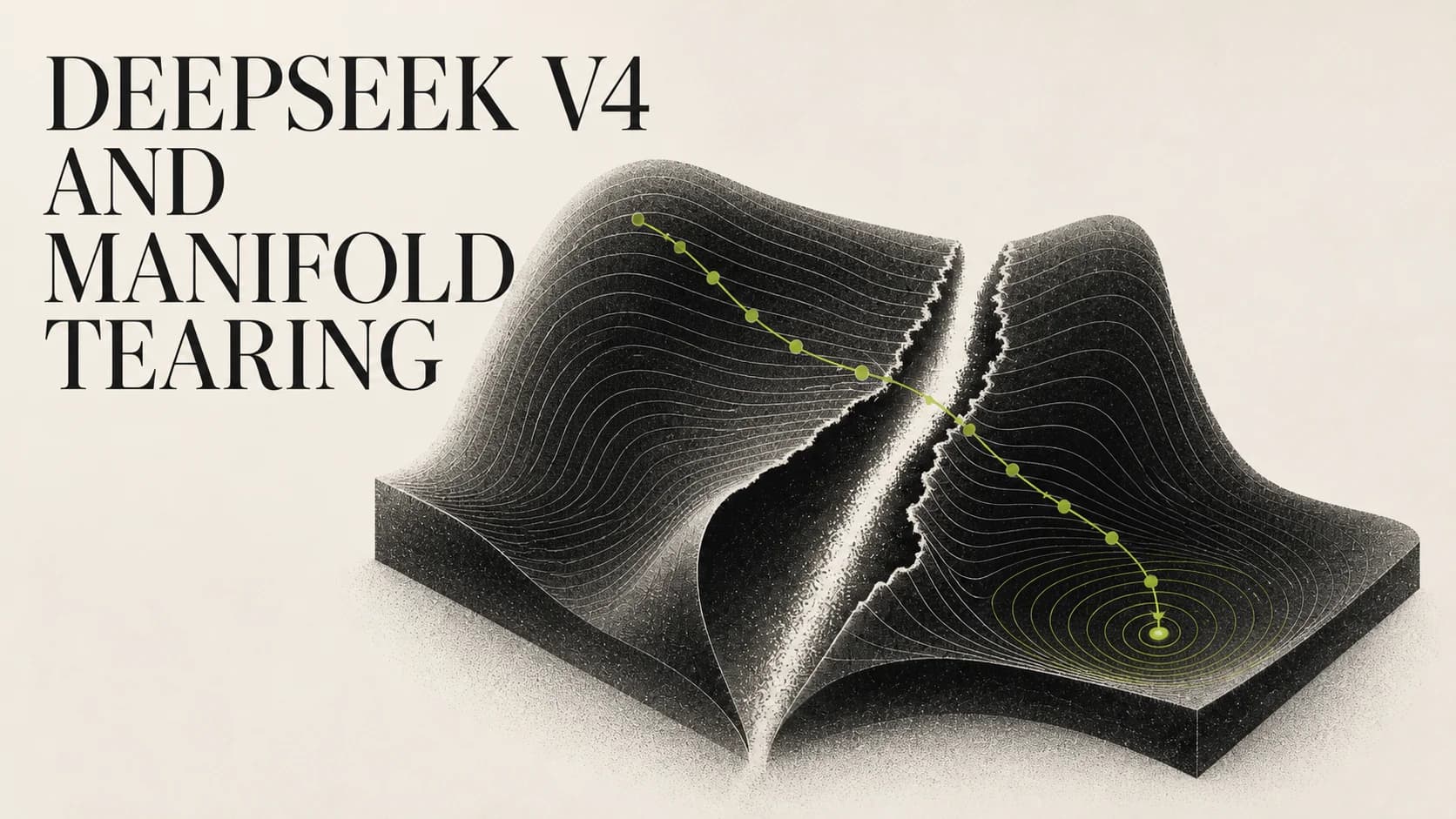
Anyone who has trained a large model has seen this scene: the loss curve drops smoothly and reassuringly, then suddenly one step shoots through the ceiling, slowly drifts back down, and leaves you with a question you don't quite know how to answer — should I rerun?

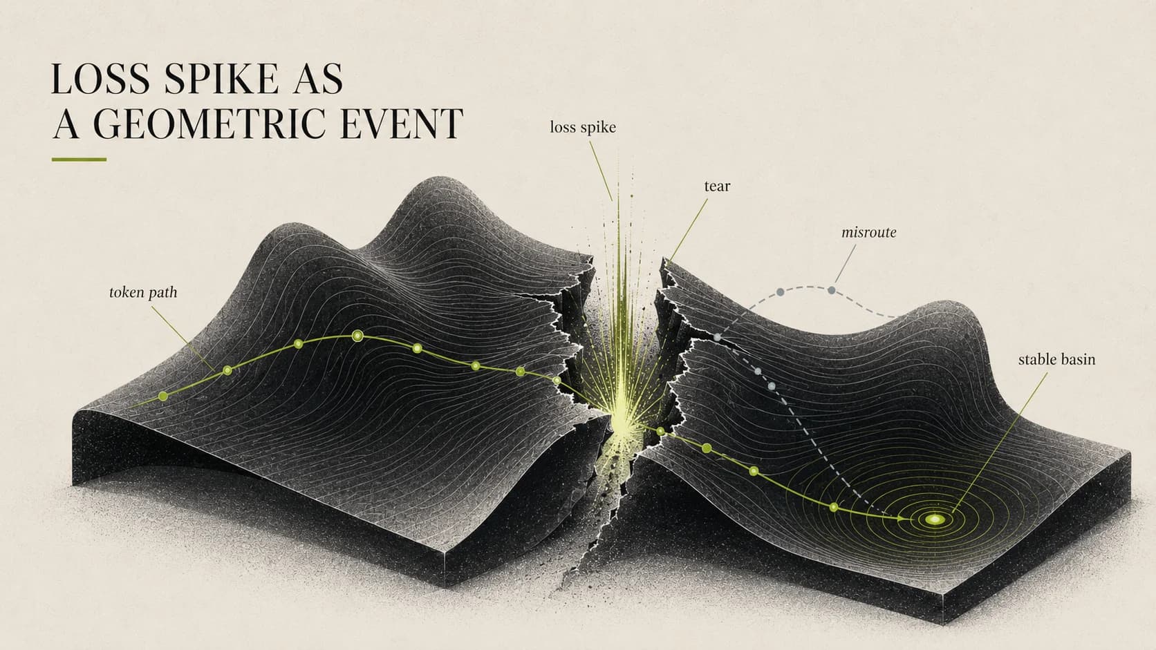
The engineering term is loss spike.

The classical story blames optimization: learning rate too high, batch went sideways, some token's gradient blew up. The community's standard treatment follows: clip the gradient, dial the LR back, restart from a checkpoint. The symptom is suppressed; the cause is left unexamined.

DeepSeek V4's tech report, plus Max Ma's geometric reading, offers a different account:

Loss spikes are not optimization failures; they are manifold tears — topological events caused by discrete routing decisions inconsistent with the local geometry.

If that holds, then V4's mHC, Anticipatory Routing, and SwiGLU clamping aren't isolated tricks. They are three patches on the same geometric problem.

1. Training a large model is an inverse problem

Lift the camera one level.

A bridge engineer with the design, materials, and load can compute whether the bridge will fail — that's a forward problem: structure given, find the result.

Training a large model is the opposite. We see data, text, and answers; we have to reverse-engineer an internal structure that could generate them. That's the textbook inverse problem.

Two things make it hard:

You don't know what the target structure looks like.
Your "solver" (the model) doesn't have a stable internal structure to begin with — it shapes itself while it solves.

That's why training large models has stayed a craft: optimizers are tried, learning rates are tried, layer counts, expert counts, router designs — all of it tried. It isn't that engineers don't want theory. It's that the thing under analysis is a moving, half-formed, high-dimensional structure feeling its way through itself.

Once you accept that, loss spike is a geometric event, not an optimization event becomes easier to swallow. In a process that solves while it shapes, the structure itself can break — not just the step size used to chase it.

2. A manifold is not a bend; a tear is not a deformation

"Manifold" sounds abstract; the fastest way in is the Earth. From space it is a sphere; standing on it, the ground under your feet looks flat. Globally curved, locally regular — that is a manifold.

The analogy carries to large models. Data isn't sprinkled uniformly across high-dimensional space; it sits on some complicated structure. Each layer reorganizes the representation, with the goal of "flattening" a tangled high-dimensional structure into something linearly separable. Olah's 2014 Neural Networks, Manifolds, and Topology is still the cleanest visualization.

The key distinction is bend vs. tear:

Bending is continuous deformation. A mountain road can be steep, but it is still connected — your map still works.
Tearing is a discontinuous jump. Two formerly adjacent points get sent to disjoint regions. The map has a slit in it.

Max Ma turned "tear" into a precise definition:

A manifold tear is a discontinuity in the layer-to-layer transport map, induced by a discrete routing decision inconsistent with the local geometry.

Note the words "discrete routing." This is exactly what MoE introduces. In a dense model, every token follows the same compute path, and there is no routing to speak of. In MoE, every layer's router makes a hard choice — and that hard choice is the entry point for "geometric inconsistency."

Tracing a single token forward, Max Ma decomposes the failure into three stages.

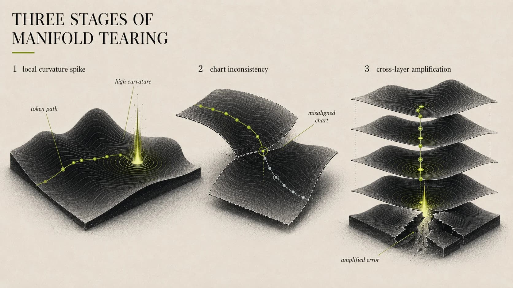
Stage 1: local curvature spike

Some activation regions develop high curvature; the second-order term stops being negligible. This is a very concrete mathematical issue: gradient descent implicitly relies on a first-order Taylor expansion

f(x + \Delta x) \approx f(x) + \nabla f(x)^\top \Delta x

When the second derivative blows up, that approximation collapses. The hiking version: the slope flips from 30° to 85°, you take your normal step, and you've stepped into the air.

Stage 2: chart inconsistency

A manifold isn't described by one global map; it is a stack of local charts.

Model parameters update at every step, and here is the catch: the router uses parameters from one step ago, $\theta_{t-\Delta t}$ , while the token now lives on $M_t$ . The chart and the geometry no longer line up — you think you're somewhere on yesterday's map, but the terrain has shifted.

In MoE that means the router sends the token to the wrong expert. Not yet a full tear, but the start of instability.

Stage 3: cross-layer amplification

A misrouted token, processed by an expert that was never trained on this part of the manifold, produces an outlier output.

If the linear transformation matrix on the residual path has spectral norm > 1, that outlier compounds layer over layer. Stack a few dozen Transformer layers, and a tiny inconsistency at layer 5 can become a loss spike at layer 50.

In the video I keep saying: what kills iterative systems isn't a single big mistake — it is a small mistake every step. This is that.

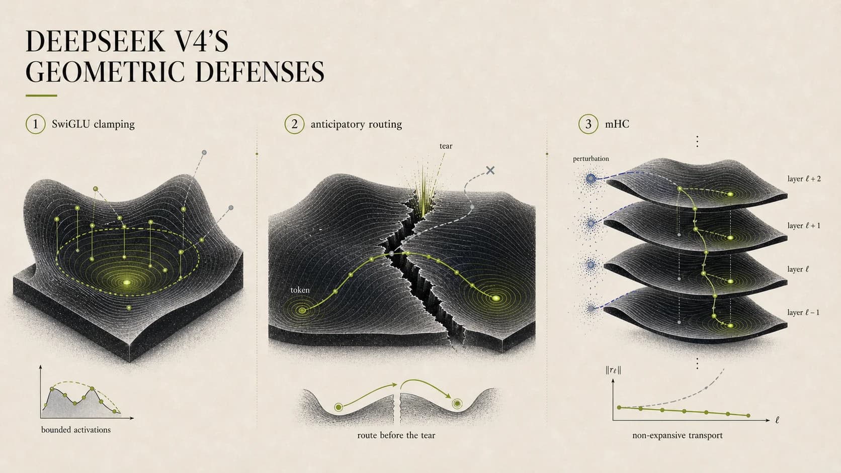
3. DeepSeek V4's three geometric defenses

V4 doesn't try to eliminate any of these stages — that's not on the table. It puts a constraint on each, so the problem doesn't run away. Max Ma's lookup table makes this clearest:

Stage	V4 mechanism	Geometric meaning
Local curvature spike	SwiGLU Clamping	Keep activations inside the chart
Chart inconsistency	Anticipatory Routing	Parallel transport from the source geometry
Cross-layer amplification	mHC	Residual is a Lipschitz-1 map

One at a time.

3.1 SwiGLU Clamping — bound the curvature inside the chart

SwiGLU has the form

\mathrm{SwiGLU}(x, g) = x \cdot \sigma(g) \cdot g

V4's move is unsubtle: clamp $x$ to [-10, 10], and clamp the gate $g$ to ≤ 10.

It sounds like a hack; the geometric reading is sharp. Any chart is only valid inside its own local range; step outside and the first-order approximation collapses. Clamping is an explicit declaration of the chart boundary — activations are not allowed to leave.

In plain terms: forget about being on the optimal path. Just don't step off the edge of the map.

3.2 Anticipatory Routing — decide using the source geometry

V4 introduces a routing design that looks strange at first: the router doesn't use the current parameters $\theta_t$ ; it uses $\theta_{t-\Delta t}$ , parameters from a step ago.

Counterintuitive on first read — wouldn't yesterday's map be less accurate for today's data?

The geometric reading clears it up. Differential geometry has a core notion called a connection: when you transport a vector from one point to another, you need a self-consistent rule. A bad rule means going around a loop and finding your vector doesn't match the one you started with — that is curvature.

What Anticipatory Routing actually does: decide using the source-point geometry, not the destination-point geometry. It accepts a small loss in apparent accuracy in exchange for temporal consistency between charts. If the chart the router sees and the chart the token actually lives on disagree at the same instant, then have the router look at a more stable, slower-changing chart.

The neat part is V4 makes this reactive. Loss starts shaking, the mechanism kicks in. Max Ma calls this "treating geometric misalignment as a detectable, correctable event."

3.3 mHC — make the residual a non-expansive map

mHC (Manifold-Constrained Hyper-Connections) is described in the V4 report as "strengthening residual connections to improve cross-layer signal stability." Max Ma writes the math out and it gets clearer.

The hyper-connection update rule is

X_{l+1} = B_l X_l + C_l F_l(A_l X_l)

In a vanilla Transformer residual, $B_l = I$ , so the spectral norm equals 1. mHC makes $B_l$ learnable, but constrains it to the Birkhoff polytope — the set of doubly stochastic matrices:

B_l \in \mathcal{M} := \{M \in \mathbb{R}^{n \times n} \mid M \cdot \mathbf{1}_n = \mathbf{1}_n,\ \mathbf{1}_n^\top M = \mathbf{1}_n^\top,\ M \geq 0\}

Every row and every column sums to 1; all entries are non-negative. The constraint is enforced via Sinkhorn-Knopp iteration — alternating row and column normalization, converging to a point inside the Birkhoff polytope.

The geometric consequence is clean: doubly stochastic matrices have spectral norm ≤ 1, so

\|B_l x - B_l y\| \leq \|x - y\|

That is Lipschitz-1, also called a non-expansive map. Meaning: residual transport from layer to layer cannot amplify a perturbation. An upstream tear can at worst preserve its size; it cannot snowball.

The input/output mappings $A_l, C_l$ get a separate treatment: forced non-negative via sigmoid, to prevent "signal cancellation producing artificial zeros" — those zeros have no geometric meaning, they are numerical artifacts.

By now you can see the three defenses are co-designed:

Clamping handles locality (don't leave the chart).
Anticipatory Routing handles time (chart at $t$ and $t+1$ stay aligned).
mHC handles space (tears don't stack across layers).

Drop any one, and the other two cannot carry the load.

4. Max Ma's deeper cut: the cause is in the data, not the architecture

If you stop here, this looks like a paper-walkthrough on V4's training stability. But Max Ma slides in a much sharper claim:

Data — not architecture — is the primary cause. Training data with a discontinuous distributional structure induces a representation manifold that was never smooth to begin with.

That sentence does a lot of damage. It implies:

mHC, Clamping, and Anticipatory Routing are all scaffolding, not the building.
They prevent an already-fractured manifold from collapsing, but they did not create the fractures.
The geometric quality ceiling is set by what you feed in.

Push it one step further. If your training data mixes samples from very distant distributions but treats them as semantically equivalent — code, natural language, math symbols, multimodal captions all in one stream — then V4's mechanisms keep training from crashing, but cannot guarantee the resulting manifold is good.

That is a harder problem than swapping architectures, and it is why I expect the next phase of competition to shift from "parameters + compute" to "data geometry."

5. Back to the Pointing-Mystery Realm: engineering evidence for the Four Realms

In The Four Realms of Neural Networks I placed training = manifold flattening at the second realm (指玄境, the Pointing-Mystery Realm), and cited Max Ma and Gen-Hua Shi's Deep Manifold framework — which formalizes this as "learnable numerical computation grounded in fixed-point theory."

That post also discussed the Muon optimizer: Newton–Schulz iteration projects each momentum update onto the nearest semi-orthogonal matrix, effectively writing "weights are geometric objects" into the optimizer.

DeepSeek V4 takes the same idea and pushes it into two new layers — forward propagation and MoE routing:

Layer	What does it	Geometric move
Optimizer	Muon	Project updates onto the isometry group (semi-orthogonal)
Routing	Anticipatory Routing	Decide in the source-point geometry
Forward residual	mHC	Constrain residual map to the Birkhoff polytope (non-expansive)
Activation	SwiGLU Clamping	Bound curvature

Four mechanisms, four positions, all doing the same kind of thing — explicitly admitting that weights and activations are geometric objects, and giving them update rules that respect that geometry.

This is the Pointing-Mystery Realm moving from "philosophical position" to "engineering default." When engineers reach for the Birkhoff polytope to constrain residual matrices, they are already thinking in geometric language — even if the paper doesn't quite say so.

Conclusion

A summary:

Training a large model is an inverse problem — structure unknown, reverse-engineered from data. Inherently unstable.
A loss spike is a geometric event — a topological tear, not an optimization blowup.
V4's three defenses (Clamping / Anticipatory Routing / mHC) constrain along the curvature, time, and space axes, scaffolding a manifold that was never smooth.
The real bottleneck is data — architecture-level stabilization is necessary, but it cannot smooth out a distribution that is intrinsically discontinuous.
The direction is converging — Muon, mHC, and Anticipatory Routing all do the same kind of thing in different positions: treat the network as a geometric object, not a bag of parameters.

At the end of the video Max Ma uses the word elegant. A model that trains stably isn't built by stacking; it is the result of modules aligning with each other — like an orchestra in tempo. Every player can be excellent and the whole performance still be noise if the timing is off. What makes V4's design interesting is that it gives this alignment a geometric grounding, not just an empirical one.

中文版 · DeepSeek V4 与流形撕裂

本文整理自我与马远老师录制的 Bilibili 对话视频《深度流形漫谈（1）—— DeepSeek V4 与流形撕裂》，并大量参考马远老师（Max Ma）在 Deep Manifold 上的原文 Single-Token Geometry: DeepSeek V4。视频是通俗版，马远老师的文章是数学版，本文把两者接到我此前在神经网络的四重境界里立的那个"流形先验"上做收口。

任何训练过大模型的人都见过这一幕：监控曲线一路下降，loss 顺滑得让人安心，突然某一步直冲天花板，然后慢慢回落，留下一个不知道该不该 rerun 的疑问。

工程上叫 loss spike。

按经典叙事，这是优化的问题：学习率太大、batch 偏了、某个 token 的梯度爆了。所以社区的常规处理是：clip 一下梯度、调一下学习率、断点续训。问题压住了，原因没人真的解释。

DeepSeek V4 的技术报告，加上马远的几何解读，提供了另一种讲法：

Loss spike 不是优化失败，是流形撕裂——一个由离散路由决策与局部几何不一致所引发的拓扑事件。

如果这句话成立，那 V4 引入的 mHC、Anticipatory Routing、SwiGLU clamping 这一组改动就不是孤立的工程 trick，而是同一道几何问题的三层补丁。

一、训练大模型是一个反问题

先把视角抬高一层。

桥梁工程师拿到设计图、材料、载荷，可以算出桥会不会塌——这是正问题：结构已知，求结果。

大模型训练正好相反。我们看到的是一堆数据、文本、答案，要反推一个能生成这些结果的内部结构。这是典型的反问题。

反问题难在两点：

你不知道目标结构长什么样；
你的"求解器"（模型）一开始也没有稳定结构，它边猜边塑造自己。

这就解释了为什么大模型训练长期是工程手艺：optimizer 要试、学习率要试、层数要试、专家数要试、router 设计要试。不是工程师不想要理论，是这件事本身就是一个动态的、还没成形的高维结构在自己摸路。

理解了这一点，"loss spike 是几何事件而不是优化事件"这个说法就比较容易接受了：在一个边塑造边求解的过程里，结构本身可以坏掉，而不只是求解步长有问题。

二、流形不是弯，撕裂不是变形

"流形"听起来抽象，但用地球理解最快：从太空看是球面，站在地面上看脚下是平的。整体可以很弯，局部可以近似规则——这就是流形。

大模型训练里类比成立：数据并不是均匀撒在高维空间，而是隐含地落在某些复杂结构上。模型每往前一层，就是在重新组织这些表示，最终目标是把一个原本缠在一起的高维结构，慢慢"展平"到可以线性分开的状态。Olah 2014 年那篇 Neural Networks, Manifolds, and Topology 至今仍是这幅图最干净的可视化。

关键在于"弯"和"裂"是两件事：

弯是连续的形变。山路再陡，路是通的，导航仍然可用。
裂是不连续的跳变。原本相邻的两点，被映射到了两个区域。地图破了一道缝。

马远把"撕裂"写成了精确定义：

流形撕裂是层间 transport map 的一个不连续点，由一次与局部几何不相容的离散路由决策诱发。

注意"离散路由"四个字——这正是 MoE 引入的新结构。Dense 模型每个 token 走一样的计算路径，不存在路由这回事；MoE 里每一层 router 都要做一次 hard 选择，这就给"几何不相容"留下了入口。

马远沿着单 token 的前向轨迹，把撕裂的发生拆成三个阶段。

阶段 1：局部曲率尖峰

某些激活区域曲率很高，二阶项不再可忽略。这是个非常具体的数学问题：梯度下降隐含地依赖一阶 Taylor 展开

f(x + \Delta x) \approx f(x) + \nabla f(x)^\top \Delta x

只要二阶导太大，这个近似就站不住。换成下山的画面：坡度从 30 度突然变成 85 度，你还按原步长迈，那一脚就踩空了。

阶段 2：坐标图不一致

流形不是一张全局地图能描述的，要靠很多局部 chart 拼起来。

模型训练时每一步都在更新参数，问题是：router 用的是上一步的参数 $\theta_{t-\Delta t}$ ，而 token 已经活在 $M_t$ 上了。chart 与几何错位——你以为自己还在旧地图上某个位置，其实地形已经变了。

具体到 MoE 里就是 router 把 token 送错了专家。还不算彻底撕裂，但已经是不稳定的开始。

阶段 3：跨层撕裂被放大

一个被送错专家的 token，被一个根本没见过这部分流形的专家处理，输出会偏离正常分布——这是一个 outlier。

如果残差路径上的线性变换矩阵谱范数 > 1，这个 outlier 会一层一层放大。Transformer 几十层堆下去，第 5 层的微小不一致，能在第 50 层变成 loss spike。

视频里我反复讲"迭代系统最怕的不是单步错，而是每一步都错一点点"——这就是。

三、DeepSeek V4 的三道几何防线

V4 不是去消灭这三个阶段——那不可能。它是在每个阶段上单独加约束，让问题不至于失控。马远的对照表把这件事讲得最清楚：

阶段	V4 机制	几何含义
局部曲率尖峰	SwiGLU Clamping	把激活夹回 chart 内
坐标图不一致	Anticipatory Routing	用源几何做平行输运
跨层撕裂放大	mHC	残差是 Lipschitz-1 映射

下面一个一个讲。

1. SwiGLU Clamping —— 把曲率夹回 chart 里

SwiGLU 的形式是

\mathrm{SwiGLU}(x, g) = x \cdot \sigma(g) \cdot g

V4 的做法很朴素：把 $x$ 限制在 [-10, 10]，把门控 $g$ 也限制在 ≤ 10。

听上去像 trick，几何意义其实很硬：任何 chart 只在它自己的局部范围内有效，超出范围一阶近似就不成立。Clamping 就是显式声明 chart 的边界——activation 不许跑出去。

用日常话讲：先别管你是不是走在最优路线上，至少别一脚踩出地图。

2. Anticipatory Routing —— 用源几何做平行输运

V4 在 router 里引入了一个看起来很怪的设计：路由判断不用当前的参数 $\theta_t$ ，而用一段时间之前的 $\theta_{t-\Delta t}$ 。

第一次看会觉得反直觉——用旧参数判断新数据，岂不是更不准？

把它放回几何里就通了。微分几何里有一个核心概念叫 connection（联络）：从一个点把向量"输运"到另一个点时，要选一种自洽的方式。错的方式，会让你绕一圈回来后向量已经不是原来那个了——这就是曲率。

Anticipatory Routing 在做的事是：在源点的几何下做决策，而不是在目标点的几何下做决策。它选择牺牲一点"看上去的准确度"，换 chart 的时间一致性。如果同一时刻 router 看到的 chart 和 token 真正所在的 chart 不一样，那就让 router 看一个更稳定、变化更慢的 chart。

更妙的是，V4 把它做成了反应式的：检测到 loss 开始抖，就启动这个机制。马远形容为"把几何错位当成一个可检测、可修正的事件"。

3. mHC —— 让残差成为非膨胀映射

mHC 是 Manifold-Constrained Hyper-Connections，在 V4 报告里被描述为"加强残差连接、增强跨层传播稳定性"。马远把数学写出来就清楚多了。

Hyper-connection 的更新规则是：

X_{l+1} = B_l X_l + C_l F_l(A_l X_l)

普通 Transformer 残差里 $B_l = I$ ，所以谱范数刚好 = 1。mHC 把 $B_l$ 换成可学习的矩阵，但强制约束在 Birkhoff 多面体上——也就是双随机矩阵的集合：

B_l \in \mathcal{M} := \{M \in \mathbb{R}^{n \times n} \mid M \cdot \mathbf{1}_n = \mathbf{1}_n,\ \mathbf{1}_n^\top M = \mathbf{1}_n^\top,\ M \geq 0\}

每行每列加起来都是 1，所有元素非负。约束的具体实现是 Sinkhorn-Knopp 迭代——交替按行、按列归一化，收敛到 Birkhoff 多面体内的一点。

这个约束的几何后果非常干净：双随机矩阵的谱范数恰好 ≤ 1，所以

\|B_l x - B_l y\| \leq \|x - y\|

这是 Lipschitz-1，又叫非膨胀映射（non-expansive map）。意思是：层与层之间的残差传播不可能放大扰动。一个上游的小撕裂，最坏只能保持原大小，不可能滚雪球。

输入输出映射 $A_l, C_l$ 还另有一招：用 sigmoid 强制非负，避免出现"信号互相抵消产生人为零点"——那种零点没有几何意义，是数值上的伪解。

到这里你应该能看出，三道防线其实是一组协同设计：

Clamping 管局部（chart 内部不出格）；
Anticipatory Routing 管时间（chart 在 t → t+1 之间对得上）；
mHC 管空间（撕裂不沿层堆叠）。

少一道，另两道也撑不住。

四、马远老师更深的一刀：根因在数据，不在架构

如果只读到这里，你会以为这就是一篇"V4 训练稳定性"的论文解读。但马远的文章里其实埋了一句更狠的话：

数据——而不是架构——才是首要原因。具有不连续分布结构的训练数据，会诱导出一个从一开始就不光滑的表示流形。

这句话的杀伤力很大。它意味着：

mHC、Clamping、Anticipatory Routing 都是脚手架，不是楼本身；
它们让一个本来就有裂痕的流形不至于崩，但裂痕不是它们造成的；
真正的几何质量上限，由你喂进去的数据决定。

往前推一步：如果你的数据里混了大量分布相距很远、但语义上被并列对待的样本（比如代码、自然语言、数学符号、多模态 caption 混训），那 V4 这套东西保的是训练能跑下去，但不可能保证最终 manifold 是好的。

这是一个比"换架构"更难的问题，也是为什么我相信下一阶段的竞争会从"参数 + 算力"转移到"数据几何"。

五、回到指玄境：Four Realms 的工程证据

我此前在神经网络的四重境界里把"训练 = 流形几何展平"放在了第二境（指玄境），并引用了马远与石根华的 Deep Manifold 框架——它把这件事数学化为"基于不动点理论的可学习数值计算"。

那篇文章里我也提到 Muon 优化器：用 Newton–Schulz 迭代把动量更新投影到最近的半正交矩阵上，本质是把"权重是几何对象"这件事写进了 optimizer。

DeepSeek V4 这次干的事，是把同一件事推进到前向传播 + MoE 路由两个新层面：

层面	谁在做	几何动作
Optimizer	Muon	更新方向投影到等距群（半正交）
Routing	Anticipatory Routing	在源几何做决策
Forward 残差	mHC	残差映射约束在 Birkhoff 多面体（非膨胀）
Activation	SwiGLU Clamping	限制曲率范围

四个机制，四个不同位置，做的是同一类事——显式承认权重和激活是几何对象，给它们配几何上自洽的更新规则。

这是指玄境从"哲学立场"变成"工程默认"的过程。当工程师不得不用 Birkhoff 多面体来约束残差矩阵时，他们其实已经在用几何的语言思考——只是论文里不一定这么写。

结论

收一下：

训练大模型是反问题——结构未知，从数据反推。这天然不稳定。
Loss spike 是几何事件——拓扑层面的撕裂，不是优化层面的爆炸。
V4 的三道防线（Clamping / Anticipatory Routing / mHC）按曲率、时间、空间三个轴分别加约束，让脚手架撑住一个本来就不光滑的流形。
真正的瓶颈在数据——架构层面的稳定化是必要的，但不会让一个有内在不连续性的数据分布变得光滑。
整个方向在收敛——Muon、mHC、Anticipatory Routing 在不同位置做着同一件事：把神经网络当几何对象，而不是参数袋。

视频末尾马老师用了"优雅"这个词。一个能稳定训练起来的大模型，不是堆出来的，是各模块之间彼此对齐的结果——像一支配合好的乐队。每个乐手再强，节拍对不上，合奏也是噪音。DeepSeek V4 这一组设计之所以有意思，是它让这种对齐有了几何上的依据，而不只是经验上的协调。